A profitable backtest with a few huge winners: inspect the concentration

A backtest can finish ahead while most trades lose money. The useful question is how the winners were earned: did the rules repeatedly capture a plausible opportunity, or did one unusual fill, oversized position, or market episode carry the result?

Profit concentration describes that dependence. It gives you a shortlist of trades to investigate, rather than a verdict that a strategy is good or bad. Start with the biggest dollar contributors, inspect their execution, and then ask whether the same opportunity appears beyond the period used to develop the rules.

A completed Bitcoin run to inspect

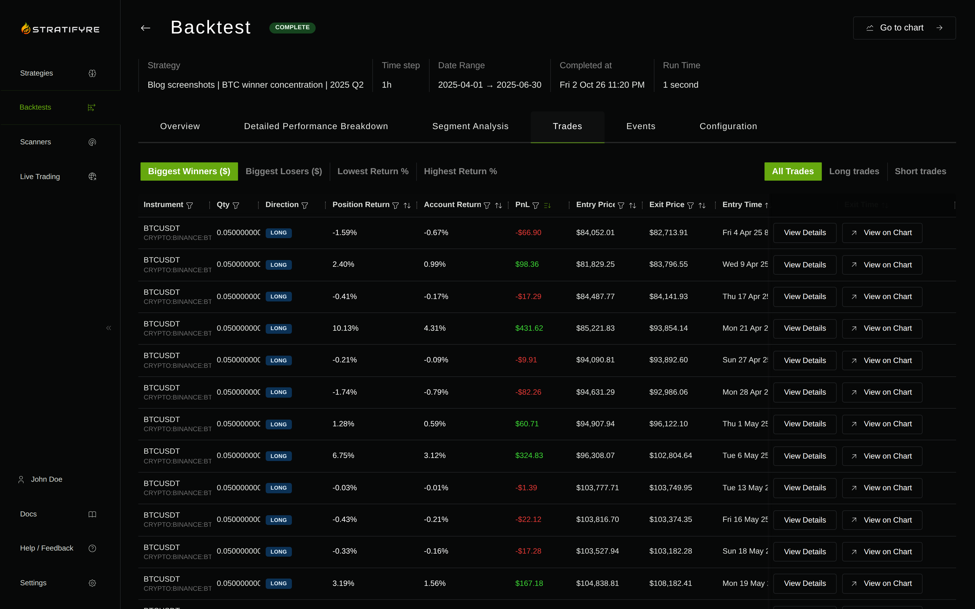
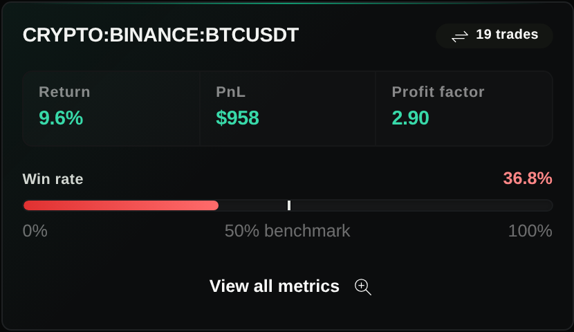
We executed an hourly EMA(20)/EMA(50) crossover on Binance BTC/USDT from April 1 through June 30, 2025. Each entry bought 0.05 BTC while flat; a downward crossover closed the holding. The run used $10,000 initial capital, on-open execution, pessimistic fills, 0.05% configured slippage, and final flattening. Its 19 completed trades reported +$958.09, with seven winners and twelve losses.

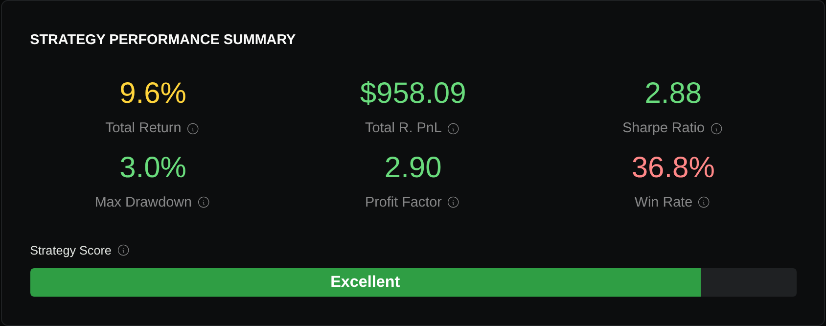
The recorded winners sum to $1,462.05; losses total $503.96. The largest winner earns $431.62: 29.5% of positive P&L and 45.0% of the $958.09 net total. These calculations use all 19 returned trade rows, rather than the first rows visible on screen. All trades use the same 0.05 BTC quantity; this example has no instrument diversification.

Start with a trade list you can reconcile

The following hypothetical worksheet contains ten completed trades across fictional instruments A, B, and C. It is arithmetic for teaching, not an executed strategy or a Stratifyre result. All amounts are USD; each row has a $20 total entry-and-exit fee. Price P&L uses assumed fills, so this example adds no separate slippage deduction. There are no open positions, funding, borrow charges, dividends, or taxes.

Trade	Instrument	Exit month	Price P&L	Fees	Net P&L
T1	A	January	+$6,000	$20	+$5,980
T2	A	February	+$1,500	$20	+$1,480
T3	B	February	+$500	$20	+$480
T4	A	January	−$400	$20	−$420
T5	A	February	−$400	$20	−$420
T6	B	January	−$400	$20	−$420
T7	B	February	−$400	$20	−$420
T8	C	January	−$600	$20	−$620
T9	C	February	−$600	$20	−$620
T10	C	February	−$800	$20	−$820

Before fees, positive price P&L totals $8,000 and negative price P&L totals $3,600 in absolute value. Their difference is $4,400; subtracting $200 of fees leaves $4,200 net. Three of ten trades win, a 30% win rate.

Metric labels need care. In trade statistics, “gross profit” can mean the sum of positive net trade outcomes, before offsetting losing trades. TradingView explicitly uses that convention and deducts configured commissions from winners. It does not mean profit before commissions. TradingView’s gross-profit definition

On this worksheet’s after-fee basis, positive trades sum to $7,940 and losing trades sum to $3,740 in absolute value. Profit factor is therefore $7,940 ÷ $3,740 ≈ 2.12, using the ratio of positive to negative trade P&L. TradingView’s profit-factor explanation

For your own report, establish whether each trade’s P&L already includes fees. Reconcile entry and exit commissions, other cash charges, open-position value, and the account-equity change before treating those figures as interchangeable. Deducting a fee twice is just as misleading as ignoring it.

Give concentration an explicit denominator

Rank the positive trades by dollar P&L on one consistent cost basis. For a chosen number of winners, calculate:

Winner share = selected winners’ P&L ÷ all positive trades’ P&L × 100%.

Here, T1 supplies $5,980 ÷ $7,940 = 75.3% of positive net trade P&L. T1 and T2 together supply $7,460 ÷ $7,940 = 94.0%. That tells you how narrowly the upside is distributed.

Another question uses a different denominator:

Signed contribution = selected trades’ P&L ÷ total signed trade P&L × 100%.

T1 contributes $5,980 ÷ $4,200 = 142.4% of the net result. There is no contradiction: the other nine trades collectively lose $1,780. Contribution can exceed 100% because losses offset the winner.

One trade carries most of the result

Ten hypothetical trades · $4,200 combined net P&L

T1 share of positive P&L

75.3%$5,980 ÷ $7,940

T1 contribution to net P&L

142.4%$5,980 ÷ $4,200

View example data

Trade	Net P&L ($)
T1	5980
T2	1480
T3	480
T4	-420
T5	-420
T6	-420
T7	-420
T8	-620
T9	-620
T10	-820

When total signed P&L is near zero, contribution percentages become unstable. A $1,000 winner divided by a $10 net result produces 10,000%; it does not indicate ten thousand percent investment return. At zero, the ratio is undefined. With a negative total, even a profitable trade has a negative signed contribution. In those cases, emphasize dollars, trade counts, and positive-winner shares instead of interpreting contribution as a quality score.

Inspect the biggest winner and the biggest loss

Use the trade list to locate the largest dollar winner, then open its chart. Repeat for the largest loss. Dollar ranking answers where the money came from; percentage-return ranking answers a different question and can elevate a tiny position with little portfolio impact.

For each extreme trade, record:

• Signal and fill: Was the entry permitted by the rules at that moment? Could the assumed order have filled at that price, given the bar interval and available liquidity?
• Exit and path: Did the exit follow the stated rules? Check gaps and the adverse movement during the holding period, not just the final gain.
• Size and exposure: Was the winner unusually large because of quantity, leverage, compounding, or a contract multiplier? Compare the risk taken at entry, not only the dollar outcome.
• Data and costs: Check splits or other adjustments where relevant, missing bars, timestamp alignment, and the charges associated with that trade.

A suspicious fill is an execution or data issue to resolve. A valid large winner is evidence about what the strategy depends on. Neither conclusion follows from its size alone.

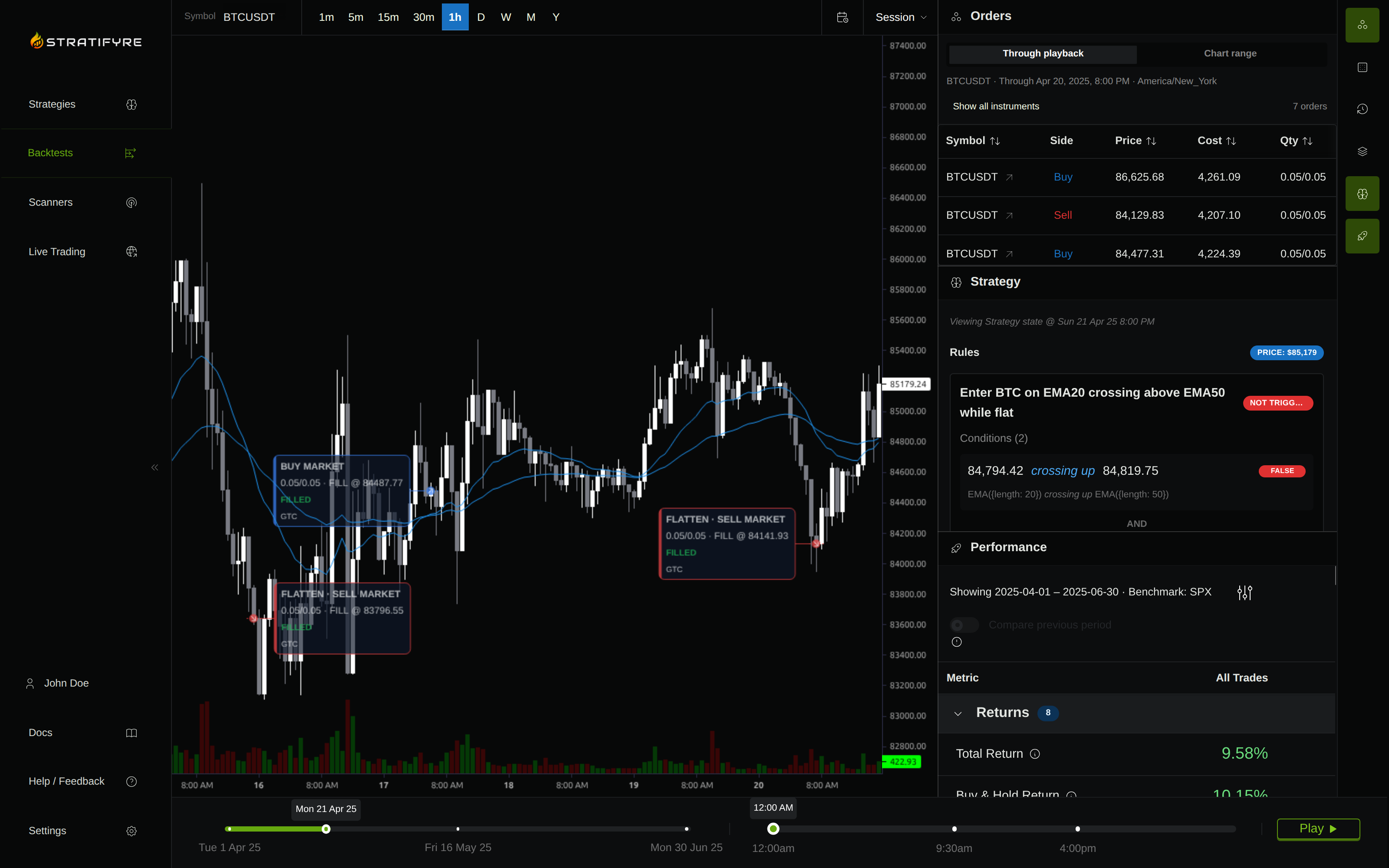
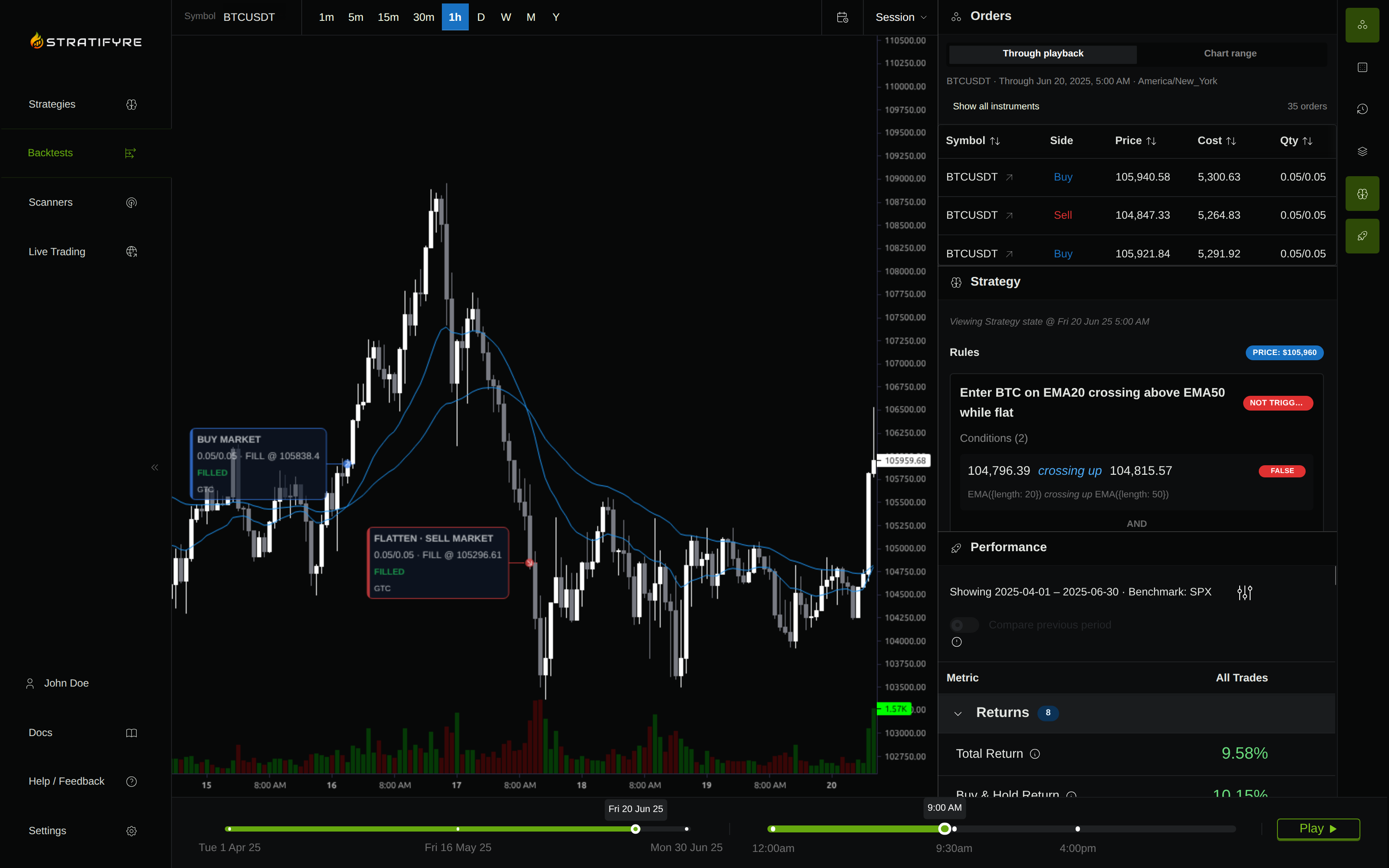
In the actual Bitcoin run, the largest winner held 0.05 BTC from April 21 at $85,221.83 to April 27 at $93,854.14, reporting +$431.62. The largest loss held the same quantity on June 20 from $106,012.66 to $103,618.77, reporting −$119.69.

Check instruments and exit periods separately

Group the same worksheet by instrument, keeping losing rows. A winners-only grouping hides the price paid to obtain the gains.

Instrument	Trades	Net trade P&L	Signed contribution
A	4	+$6,620	157.6%
B	3	−$360	−8.6%
C	3	−$2,060	−49.0%
Total	10	+$4,200	100.0%

A carries the result; B and C reduce it. That prompts a question about the strategy’s opportunity and exposure across instruments. It does not justify selecting A after seeing the answer and presenting the selection as an independent discovery.

Grouping by exit month gives January +$4,520 and February −$320. These are completed-trade totals booked at exit. A trade opened in December and closed in January belongs to January in an exit-month analysis; its entire P&L is assigned there. That does not show how much account equity moved during January while the trade was open.

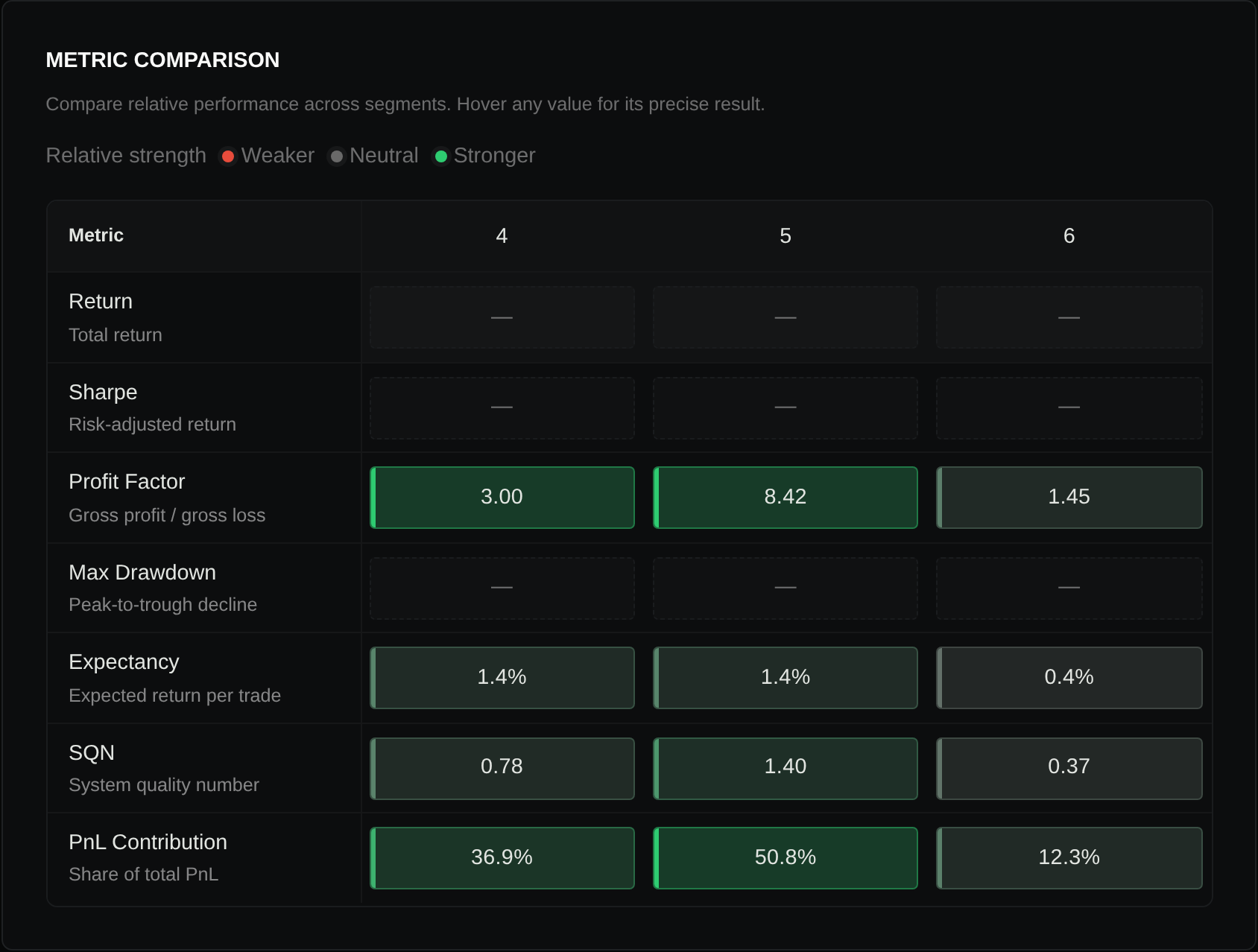
Stratifyre documents instrument and exit-month/quarter segment analysis. Treat those as separate views of the same trades: adding instrument contributions to month contributions would count the same P&L twice. A curve accumulated from closed-trade P&L is also different from a portfolio curve that marks open positions and accounts for cash costs throughout the run.

Remove a winner only as a diagnostic

Subtracting T1 from the worksheet leaves $4,200 − $5,980 = −$1,780. Subtracting T1 and T2 leaves −$3,260. These calculations answer: “How much did these observed rows support the total?”

They do not answer: “What would the portfolio have earned without those trades?” Removing an earlier position can change available capital, subsequent sizing, exposure limits, overlapping positions, and later decisions. A genuine alternative portfolio requires a new run with a rule that could have excluded the trade using information available at the time.

Keep the original rows and label any subtraction worksheet as a diagnostic. Avoid calling it an adjusted backtest, corrected equity curve, confidence score, or native top-N exclusion feature.

Test the opportunity beyond the selected winners

A strategy that limits losing trades while allowing gains to run can have a low win rate and depend on infrequent large gains. Removing those gains mechanically can remove the very outcome its rules seek. Hurst, Ooi, and Pedersen’s original trend-following research studies time-series momentum across a long history and multiple markets; it provides context for evaluating a strategy family, rather than validation of this worksheet or your particular rules. A Century of Evidence on Trend-Following Investing

Ask whether the dominant winners come from independent opportunities or one shared episode. Ten profitable positions during the same market shock may provide less variety of evidence than their row count suggests. Ten trades in total are enough to explain this arithmetic, but provide little basis for estimating how often its large winner might recur.

Before revising rules, reserve a later period that you have not used for strategy decisions. Freeze the instruments, entry and exit rules, sizing, fill assumptions, and cost model; then compare the later trade list, losses, and concentration. Retain an unfavorable result. If you alter the strategy after studying that period, it becomes development data and you need fresh evaluation evidence.

Your review should end with a concrete finding: a data problem to fix, an exposure dependence to investigate, or a plausible but sparsely observed opportunity requiring more evidence. A high concentration percentage alone cannot make that decision.

Open the Segmented Performance guide and inspect the trades and instruments contributing most to your backtest P&L, with their losses and cost basis alongside them.