Grid versus random search: budget your strategy tests first
Count parameter combinations, compare searches at a matched trial budget, and separate historical candidate selection from later validation.
Four indicator periods and four entry thresholds create 16 candidate strategies. Add three stop distances and three profit targets, and the search becomes 144 candidates. The extra settings multiply the workload before you have learned whether they improve the strategy.
Grid search and randomized parameter search offer different ways to spend that workload. Choose between them by defining the parameter domain, a trial budget, and a selection rule first. Neither method turns the highest historical return into evidence of future profitability.
The planning counts and scatter diagram below are illustrative examples. A separate completed three-attempt comparison at the end shows actual product results; no measured speed comparison is claimed.
Count the grid before choosing a method
A grid evaluates every combination of the values you specify for each parameter. It is exhaustive over those lists, rather than over every possible value between their endpoints. This is the definition used by scikit-learn’s ParameterGrid.
For a hypothetical RSI-based strategy, start with two parameters:
| Parameter | Candidate values | Count |
|---|---|---|
| RSI period, in bars | 10, 14, 18, 22 | 4 |
| Entry threshold, RSI points | 20, 25, 30, 35 | 4 |
Grid trials = distinct period values × distinct threshold values = 4 × 4 = 16.
Adding three stop distances and three targets produces 4 × 4 × 3 × 3 = 144 trials. Repeating that search across several training windows adds another multiplier. Reserve separate runs for the unchanged baseline and later validation; do not hide them inside the search count.
Count the actual values after rounding. Five requested points inside a narrow integer range can collapse into fewer than five distinct periods. Also check which numeric constants vary: an indicator period, an entry threshold, and a position quantity answer different research questions. Changing sizing along with entries makes interpretation harder.
What random search changes
Random search draws candidate settings from declared lists or distributions until it reaches a fixed attempt budget. That gives you a way to explore a broad domain without evaluating its complete grid.
The original Bergstra and Bengio random-search paper studied machine-learning hyperparameters. Its practical insight is that a grid can spend many trials repeating values along a parameter that matters most, while randomized draws can explore more distinct values along that dimension. That motivates trying random search when you do not know which settings matter. The paper does not establish which method produces better trading strategies.
Same 16-point budget, different coverage
Illustrative parameter locations · Shared bounds from 0 to 1
16 locations · Four distinct values on each axis
16 locations · More distinct values along each axis
View example data
| Parameter A | Parameter B |
|---|---|
| 0 | 0 |
| 0 | 0.3333 |
| 0 | 0.6667 |
| 0 | 1 |
| 0.3333 | 0 |
| 0.3333 | 0.3333 |
| 0.3333 | 0.6667 |
| 0.3333 | 1 |
| 0.6667 | 0 |
| 0.6667 | 0.3333 |
| 0.6667 | 0.6667 |
| 0.6667 | 1 |
| 1 | 0 |
| 1 | 0.3333 |
| 1 | 0.6667 |
| 1 | 1 |
| Parameter A | Parameter B |
|---|---|
| 0.07 | 0.88 |
| 0.28 | 0.69 |
| 0.49 | 0.84 |
| 0.69 | 0.58 |
| 0.92 | 0.91 |
| 0.14 | 0.39 |
| 0.33 | 0.23 |
| 0.57 | 0.41 |
| 0.81 | 0.12 |
| 0.95 | 0.33 |
| 0.19 | 0.09 |
| 0.41 | 0.55 |
| 0.63 | 0.14 |
| 0.74 | 0.82 |
| 0.86 | 0.49 |
| 0.09 | 0.63 |
The sampling rule matters. Drawing periods from integers 10 through 22 explores a different set from drawing only 10, 14, 18, and 22. Drawing thresholds continuously between 20 and 35 differs from drawing only the four table values. Specify which comparison you intend: identical finite candidate lists, or different coverage of the same bounded domain.
With identical finite lists and sampling without replacement, drawing all 16 combinations eventually evaluates the same candidate set as the grid. With replacement, some attempts repeat settings. ParameterSampler explicitly distinguishes these cases: list-only inputs use sampling without replacement; introducing a distribution uses sampling with replacement. These are that library’s rules, not a promise about another optimizer.
Compare methods at a matched budget
Comparing 144 grid evaluations with 16 random draws confounds the method with the amount of research. Begin with equal attempt budgets and record distinct candidates separately.
For the two-parameter example, a useful plan is:
| Budget item | Grid plan | Random plan |
|---|---|---|
| Search attempts | All 16 listed combinations | 16 declared draws |
| Unique settings | 16, if lists remain distinct | Count actual sampled settings |
| Training baseline | One shared run | Same baseline result |
| Later validation | One frozen selection | One frozen selection |
| Later baseline | One shared run | Same baseline result |
This illustrative plan totals 36 planned attempts: 32 search attempts, one shared training baseline, two selected-candidate runs on the later window, and one shared baseline run on that later window. Budget any retries separately.
Keep the instrument set, venue, bars, dates, warmup, entry/exit logic, signal and fill timing, capital, sizing, fees, slippage, and session rules identical. For futures, include contract/roll assumptions; for perpetuals, include funding. Candidate settings should be the only intended change.
Equal trial counts do not guarantee equal elapsed time or cost. Some parameter choices produce more trades or require more history. Record failures, cancellations, duplicates, completed attempts, elapsed time, and actual charges separately. A failed attempt still consumed resources even if it contributed no usable score.
Set the stopping rule in advance: the attempt limit plus a time or spending limit. If one method stops early, report the smaller completed budget. Do not keep rerunning random seeds until one produces an attractive winner. If you plan several seeds, include every seed’s attempts in the total budget and report the spread of outcomes.
What Stratifyre’s parameter fuzzing means here
Stratifyre documents grid and Monte Carlo optimization within walk-forward analysis. Its Monte Carlo documentation distinguishes Auto parameter perturbation, which changes settings and reruns historical backtests, from Bootstrap trade resampling.
Parameter fuzzing is the relevant comparison for this article. It changes strategy inputs while using historical market data. A distribution of those candidate results is not a distribution of future returns, a simulated market forecast, or a trade-bootstrap experiment.
The inspected parameter-search implementation generates a configured number of randomized variants and can repeat identical settings. Grid generation deduplicates rounded values before counting combinations. Consequently, the same numerical budget can produce different counts of unique candidates. Save sampled parameter values and the effective seed; a seed alone is insufficient if the rules, data, or search settings later change.
Verify admissible ranges and the actual generated settings before treating the searches as comparable. Default perturbation and explicit range overrides need not cover the same values, and rounding can change coverage. This guide does not establish a current production UI control or demonstrate an executed optimizer benchmark.
Choose the objective before looking at results
Write one objective and a screening policy before evaluating candidates. An illustrative policy might rank net return after costs while requiring at least 40 closed trades and a maximum drawdown no larger than 15%. Those thresholds are a research example, not validated risk limits.
Treat screening and ranking as separate operations. A high-return candidate that violates your drawdown limit does not qualify simply because it tops the return column. If the optimizer cannot enforce your screening conditions before ranking, retain all trials and apply those conditions separately.
Stratifyre’s inspected walk-forward selector maximizes its configured objective and retains the first evaluated candidate when objective values tie. That selection alone does not enforce the illustrative trade-count or drawdown conditions above. Check the selected candidate’s complete report, including missing metrics and zero-trade cases, before using it for validation.
Keep every candidate’s parameters, objective value, costs, trade count, drawdown, and selection status. Preserve losing and unselected results. A winner without its search history hides how many chances you gave yourself to find it.
Validate the selection on a later window
Freeze one selection from each method using the training-window rule. Then evaluate both on the same later window that did not guide parameter choice. Keep the baseline alongside them and preserve negative results.
Bailey and colleagues’ backtest-overfitting paper explains why repeated strategy selection can fit historical noise and why a holdout alone does not account for the number of trials. Later-window testing adds evidence; it does not erase the search history or prove a strategy will work live.
If you redesign settings after seeing that later window, it has become development data. Record the additional trials and reserve another untouched evaluation period. A fair comparison needs a fixed research procedure, not two carefully chosen best runs.
Actual product comparison: three attempts each
We executed two separate walk-forward analyses in the demo account with an equal budget of three training candidates each. Both used Binance BTC/USDT hourly bars, January 2025 training and February 2025 later testing, $10,000 fixed capital, 0.05 BTC entries, on-open execution, pessimistic fills, final flattening, 0.10% configured crypto commission and 0.05% slippage. The only selected numeric occurrence was the entry EMA length, Entry.C0.0; the entry slow EMA(50), exit EMA(20)/EMA(50), and position sizing stayed fixed.
The declared domain was integer lengths 18 through 22. The three-point grid evaluated 18, 20 and 22. Three seeded random draws evaluated 18, 20 and 19, using seed 20261002. This compares different coverage of the same bounds, not sampling the identical finite grid list. All six attempts completed; each method had three unique settings in this draw. These results do not reproduce the hypothetical RSI experiment above.
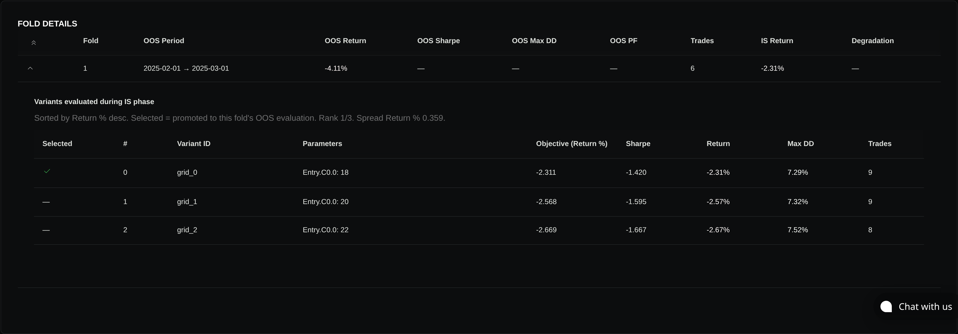
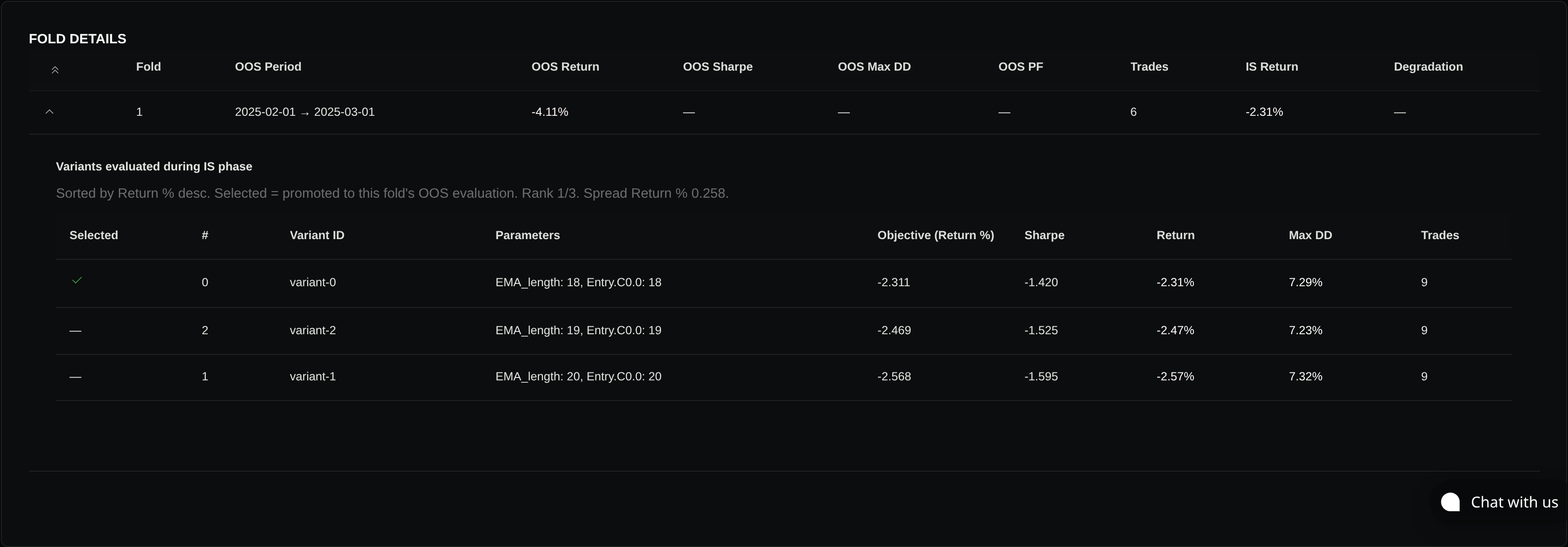
EMA_length display key accompanies the exact selected path; it does not mean the exit EMA also varied.| Method | Training lengths in evaluation order | Selected length | Selected January return | February test return | February trades |
|---|---|---|---|---|---|
| Grid | 18, 20, 22 | 18 | −2.3106% | −4.1061% | 6 |
| Seeded random | 18, 20, 19 | 18 | −2.3106% | −4.1061% | 6 |
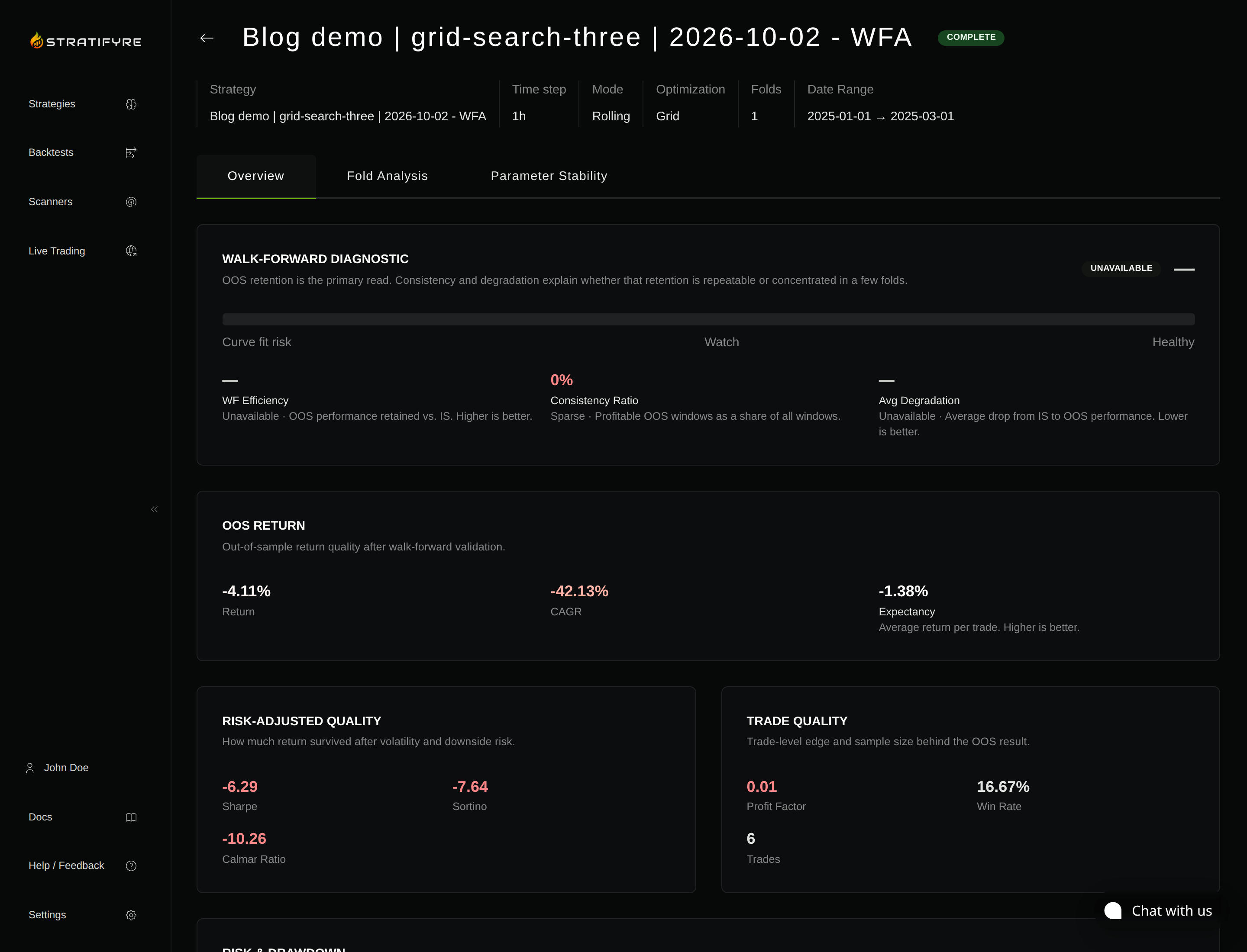
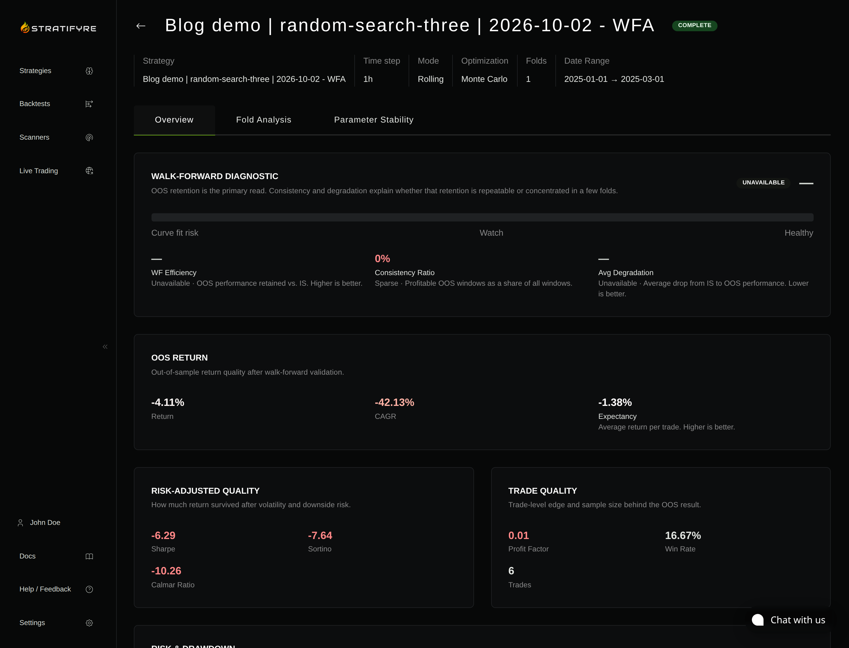
The later-window evidence comes from the actual WFA reports: ordinary backtest URLs for the persisted OOS child IDs returned “Backtest not found.” Missing fold risk metrics and unavailable efficiency/degradation values remain disclosed. We did not measure elapsed-time advantage, actual charges, verified warmup coverage or per-fill commission reconciliation; configured costs are not proof of charged costs. This bounded comparison uses six search attempts plus two selected-candidate tests; it does not execute the larger 36-attempt teaching plan or add its separate baseline controls.
Use a small grid when you can afford every combination and need transparent coverage of specific settings. Consider randomized search when the complete grid exceeds your budget and you can define meaningful sampling rules. Before launching either, write the candidate budget and separate validation window into your experiment plan; the backtesting guide provides the configuration context.
Put your strategy rules to the test
Build your strategy, inspect historical trades, and review the assumptions behind your results.
Build and test your strategy