Parameter sensitivity: check the neighborhood around your best backtest

Your best backtest uses a 20-bar lookback. What happens at 18 or 22 bars? If a small change destroys the result, the exact setting deserves investigation before you rely on it.

Parameter sensitivity asks how much behavior changes around an existing candidate. The aim is to understand that candidate, not keep replacing it with whichever neighbor earns the most. A broad historical plateau can be encouraging, but it does not establish an economic edge, rule out overfitting, or predict future profitability.

The two-parameter settings and plateau/spike scores below are hypothetical teaching examples. A separate three-setting Bitcoin demonstration supplies the actual product screenshots and return chart; it varies only the entry EMA length.

Freeze the candidate before checking its neighbors

Write down the strategy you are investigating and why its rules might make economic sense. Include the original selection history: different settings, instruments, timeframes, exits, and discarded ideas all matter. Bailey and colleagues explain how repeated selection among backtests creates false-positive risk; reporting only the winning configuration hides part of that process. The Probability of Backtest Overfitting.

Keep the base rules, instrument universe, venue, interval, and date window fixed for the first comparison. Also fix capital, position sizing, fees, slippage, signal/fill timing, and treatment of open positions at the window end. Record sessions, timezone, and any corporate-action or contract-roll assumptions that apply. Otherwise, a changed fill model or larger position can masquerade as a parameter effect.

Choose one main comparison metric before rerunning anything, such as return after modeled costs. Pair it with risk and activity checks rather than ranking by return alone. Predefine what would trigger investigation: a drawdown beyond your risk limit, a sharp collapse in trade count, or a large deterioration in the main metric. There is no universal cutoff that makes a neighborhood robust.

Define a small, meaningful neighborhood

For illustration, suppose the candidate has a 20-bar indicator lookback and a stop distance of 2.0% from entry. These are settings to inspect, not a complete trading strategy.

Parameter	Base	Predefined nearby values
Lookback	20 bars	18, 20, 22 bars
Stop distance	2.0%	1.8%, 2.0%, 2.2%

Testing every combination gives 3 × 3 = 9 configurations: the base plus eight neighbors. Count unique configurations separately from repeated execution of the same configuration. A new base rerun can check reproducibility; it is not a tenth distinct setting.

Use integer values for bar counts and valid ranges for thresholds. Respect relationships between parameters: a fast moving average should remain faster than the slow average if that is part of the strategy definition. Check that the tool changes the intended occurrence of a setting, especially when the same number appears in several rules.

One parameter at a time helps isolate causes. A small two-parameter grid adds the corners, where interactions may appear. More dimensions grow quickly: three choices for four parameters create 81 configurations. Set a run budget and stop rule in advance; do not expand the grid whenever its boundary contains a tempting result.

Read a plateau and a spike carefully

In an invented plateau, neighboring settings might behave similarly. In an invented spike, the center might stand far above all eight nearby values. The second shape prompts a concrete question: which trades or rule decisions changed when the lookback or stop distance moved?

Here is a compact summary of the two entirely synthetic nine-setting neighborhoods:

Arbitrary score	Plateau example	Spike example
Base setting	10.00	10.00
Median of eight neighbors	9.65	1.90
Lowest neighbor	9.40	1.50
Base minus lowest neighbor	0.60	8.50

The last row uses a simple descriptive calculation:

Gap = base score − lowest score among the eight neighbors.

For the plateau, 10.00 − 9.40 = 0.60 score units. For the spike, 10.00 − 1.50 = 8.50. This is a summary of these invented values, not a statistical test or a probability of future failure. When using real returns, report the difference in percentage points rather than calling it a percentage decline.

A smooth patch can still be consistently unprofitable after costs. Nearby settings can also trade almost identically, so eight neighbors are not eight independent confirmations. And a sharp discontinuity may have an understandable cause, such as a threshold excluding a few large trades. Shape is a diagnostic clue; the trade record supplies the explanation.

Compare trades, exposure, and costs

Keep one row per completed configuration, including unfavorable outcomes. Alongside your chosen metric, record:

• Maximum drawdown: did a similar return require a much deeper equity decline?
• Trade count: did a neighbor stop trading, or did one additional trade explain the difference?
• Exposure and sizing: did time in positions or capital at risk change?
• Turnover and costs: did extra trades consume the apparent improvement?
• Concentration: did most of the result come from one instrument, trade, or short period?

Inspect trades around the largest differences. For a lookback change, compare the signal time and eventual fill. For a stop change, inspect the affected exits and whether sizing changes with stop distance. If risk-based sizing does change, the comparison includes that exposure effect; record it instead of attributing everything to the exit rule.

Record missing data and failed runs without inventing scores. Keep completed no-trade configurations visible, including any legitimately reported zero return; distinguish unavailable metrics from measured zeros. A neighborhood with incomplete coverage cannot support the same conclusion as nine comparable completed runs.

Separate diagnosis, validation, and the final test

The neighborhood on the original research window diagnoses local sensitivity. It does not turn that window into unseen data. Model-selection guidance makes the same distinction: settings used during development need evaluation on data excluded from that selection. scikit-learn’s development and evaluation guidance.

Use three explicit roles for your timeline:

1. Development: choose the candidate and define its neighborhood, metrics, and decision rules.
2. Later validation: run the frozen candidate and predefined neighborhood on a later window to investigate whether behavior persists. Any revisions based on these results make this window part of development.
3. Untouched final test: evaluate the frozen final specification once on a separate period that did not guide those revisions. Keep its results out of further tuning.

Use chronological windows for this exercise. Randomly shuffling nearby market observations can undermine the separation between development and evaluation; scikit-learn documents this problem for correlated time-series data. Time-series cross-validation.

Provide enough preceding history for the longest indicator lookback, while excluding warmup activity from the scored window. Define how positions and account state begin and end in each window. Compare windows with their durations and trade counts visible; short, sparse periods may offer little evidence.

An untouched test is another check, not a cure for every research bias. Bailey and colleagues also discuss why holdout evidence alone does not account for the number of alternatives tried. If you change the strategy after seeing the final test, it becomes development evidence and another untouched evaluation is needed.

Turn the check into a research decision

A useful outcome is a documented explanation: the candidate remained similar across the planned neighborhood, failed a predefined constraint, or depends on a few identifiable trades. Preserve the original candidate and every comparison result. A search tool selecting a winner does not remove the need to inspect the other configurations.

For a fragile result, investigate the mechanism or simplify the rule before launching a wider search. For a stable result, keep testing costs, data assumptions, and later behavior. Neither outcome justifies selecting a new winner from every diagnostic check.

Actual product example: three entry lookbacks

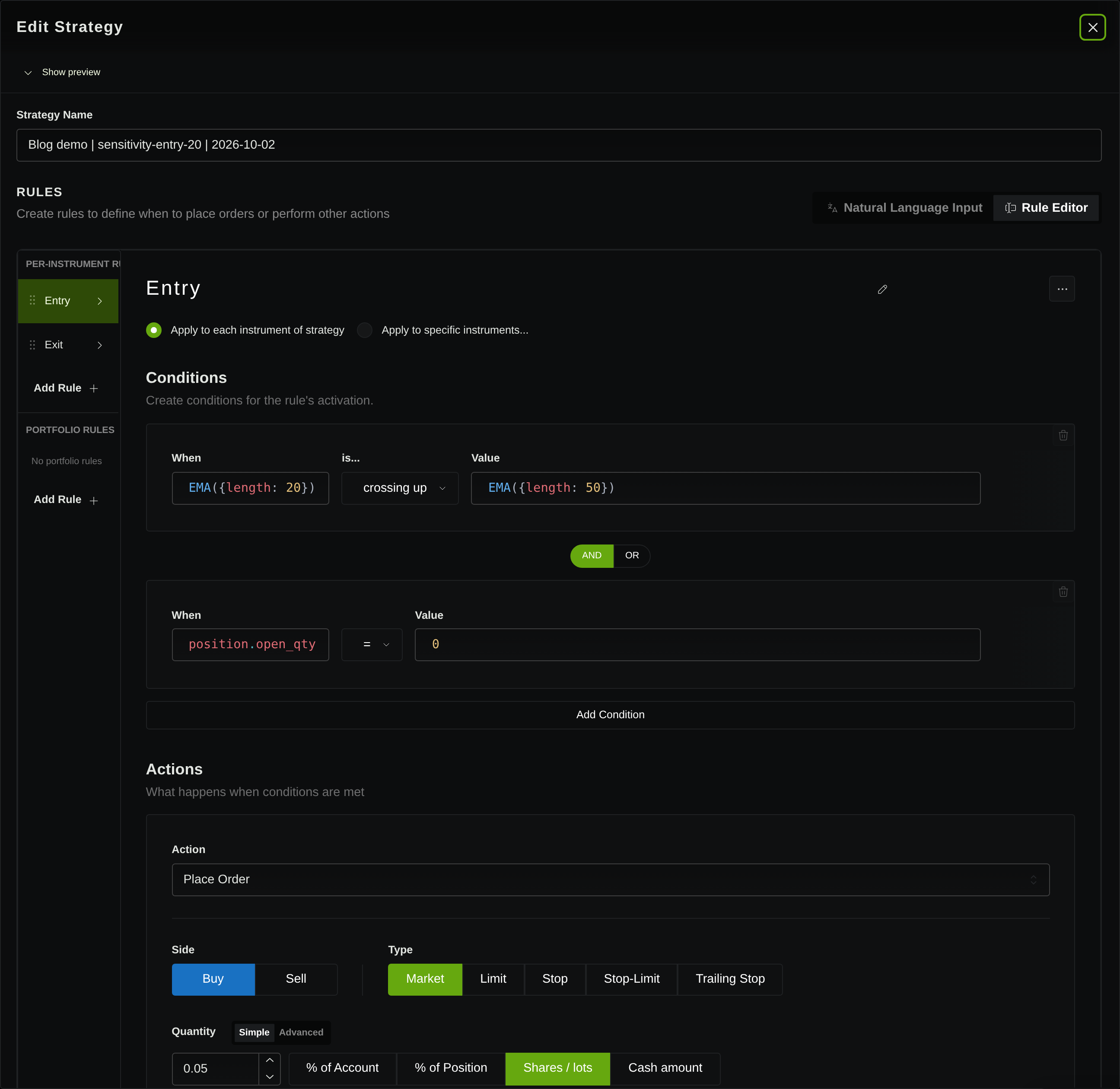
We saved and executed three separate strategies in the demo account using Binance BTC/USDT hourly bars from January 1 through March 31, 2025. The baseline enters 0.05 BTC on an EMA(20) crossing above EMA(50) while flat; neighbors change only that entry lookback to 18 or 22. Every exit keeps EMA(20) crossing below EMA(50). Each run uses $10,000 capital, on-open execution, pessimistic fills, final flattening, 0.10% configured crypto commission and 0.05% slippage. There is no stop-distance dimension in this smaller demonstration, so it does not execute the nine-setting teaching neighborhood above.

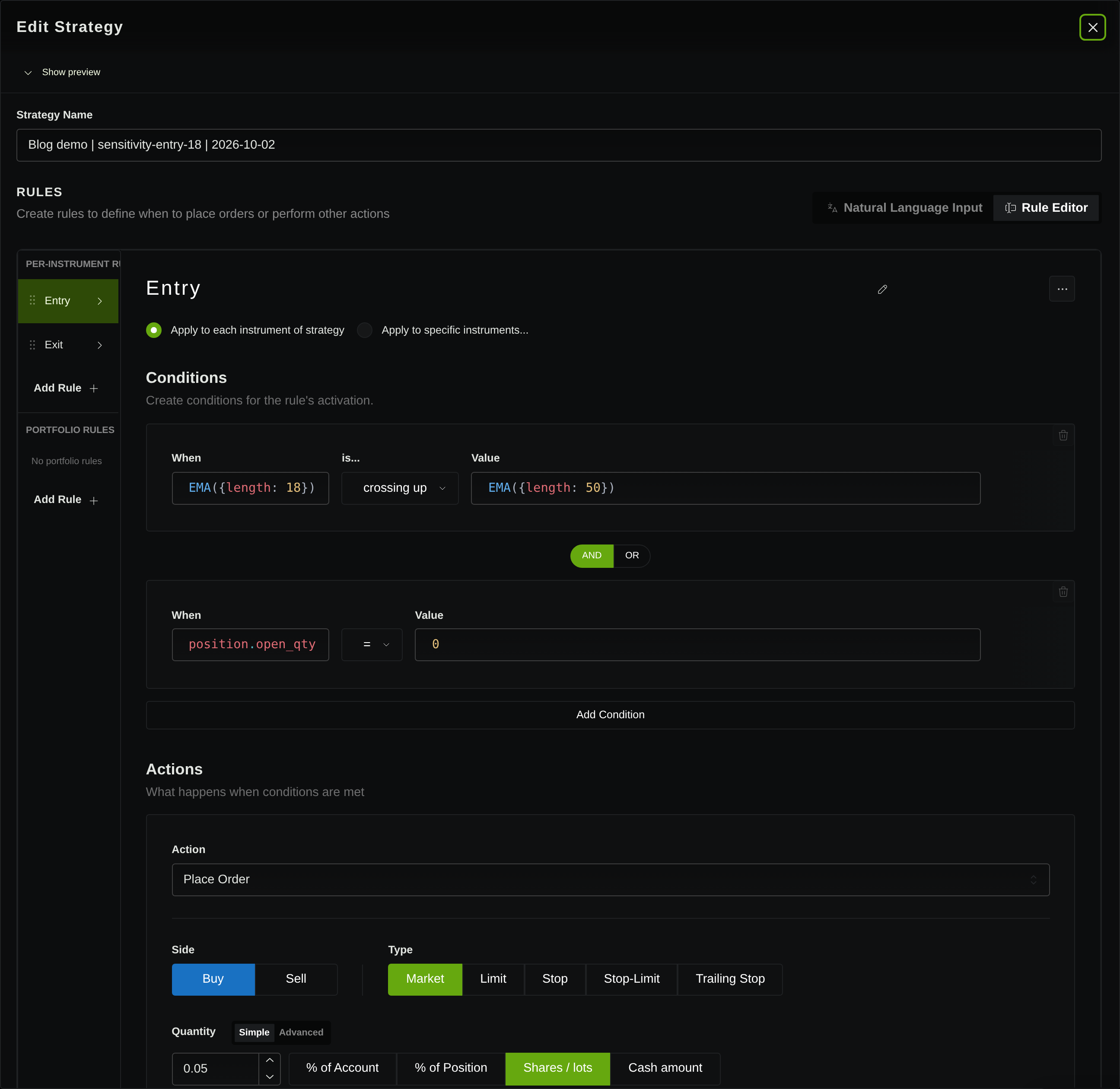
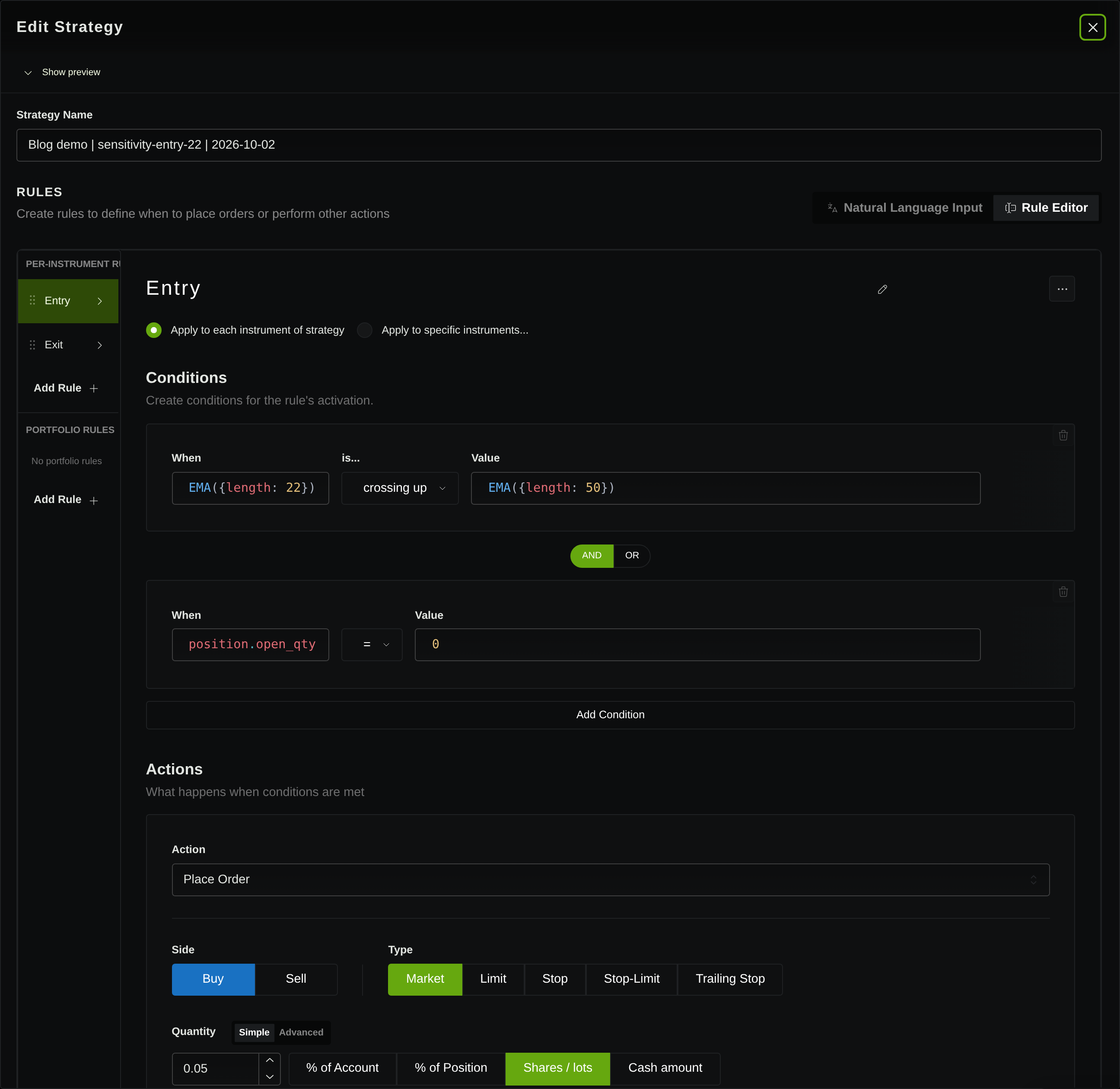
Entry EMA length	Return	Net P&L	Ending equity	Max drawdown	Trades	Exposure
18	−6.5379%	−$653.79	$9,346.21	12.0334%	24	41.6204%
20, baseline	−6.7579%	−$675.79	$9,324.21	12.1388%	24	39.8611%
22	−7.7891%	−$778.91	$9,221.09	13.3939%	23	39.2130%

Actual one-parameter neighborhood

Three completed Bitcoin backtests · January–March 2025

Return (%)Max drawdown (%)

All three completed settings lost money · Baseline return −6.7579%

Maximum drawdown increases from 12.0334% to 13.3939% across these settings

View recorded data

Recorded return (%)

Fixed exit EMA / Entry EMA	18	20	22
20	-6.53787430000004	-6.7579092625	-7.7890988199999995

Recorded maximum drawdown (%)

Fixed exit EMA / Entry EMA	18	20	22
20	12.033432614930884	12.138822354453598	13.393860652975576

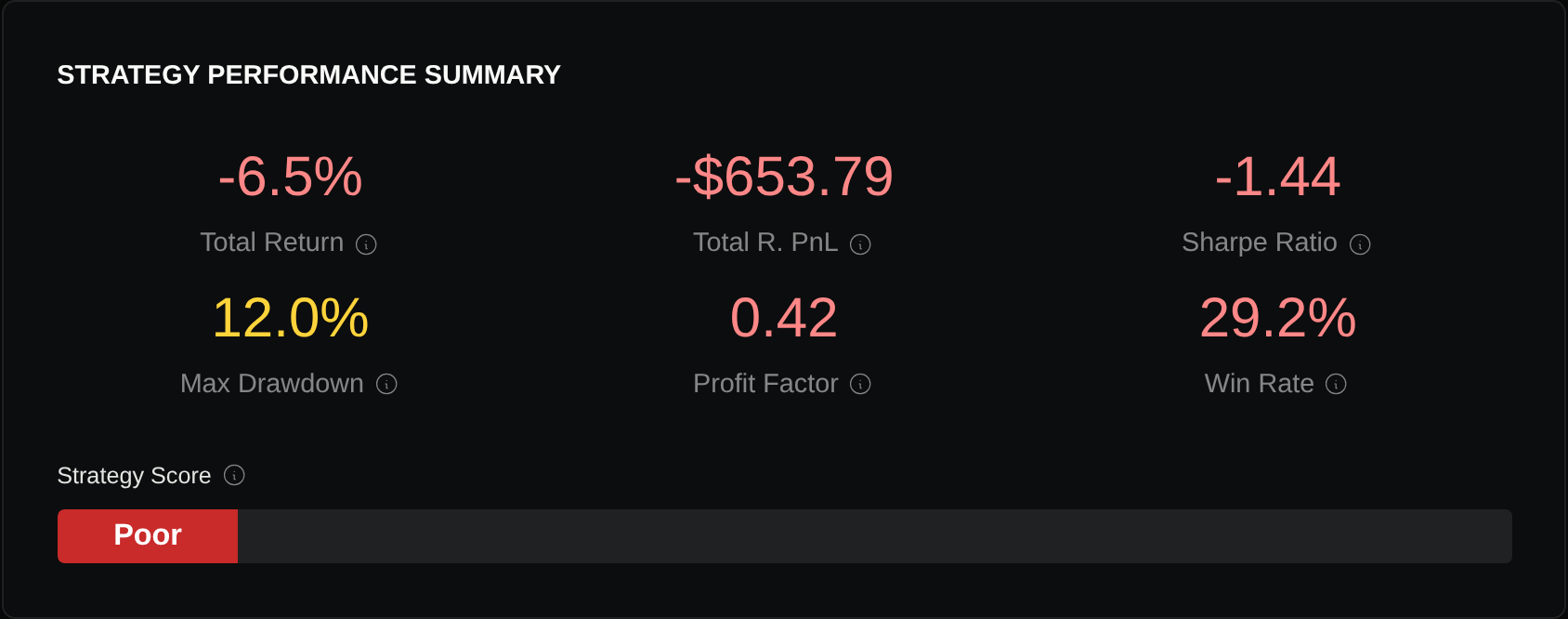
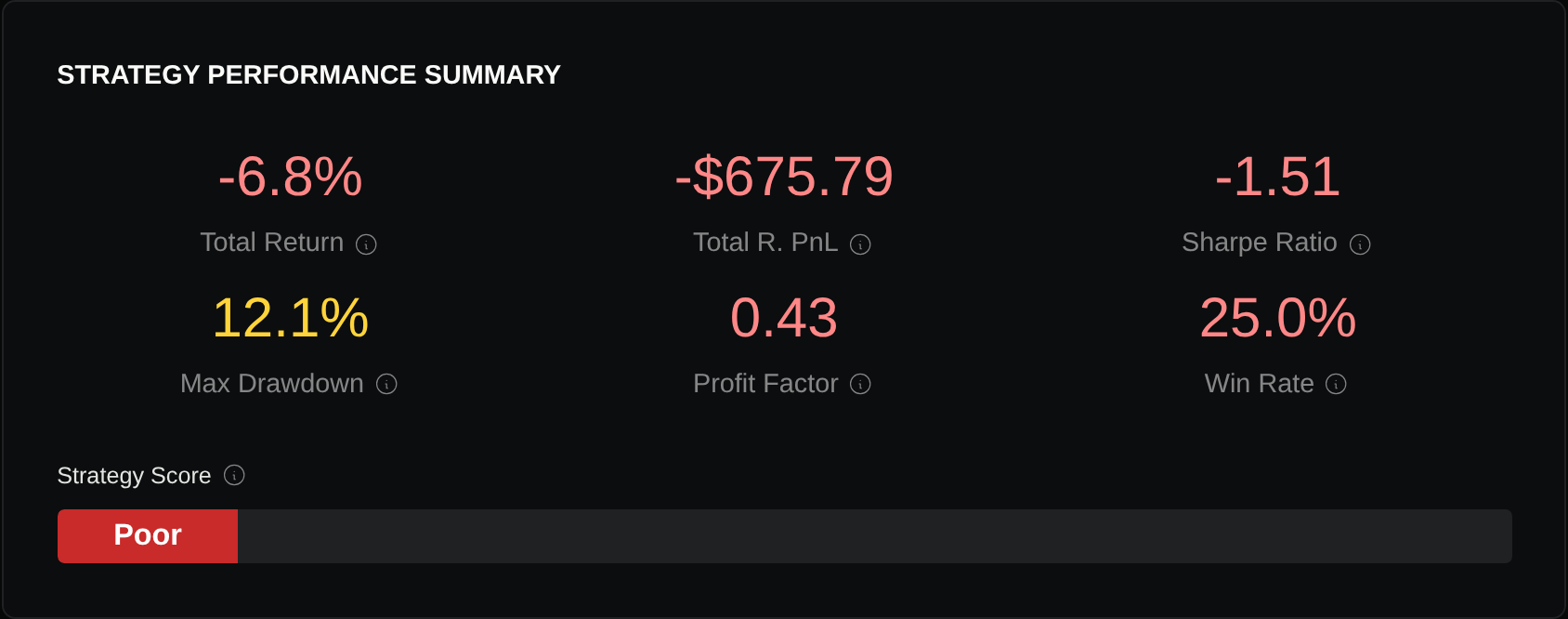
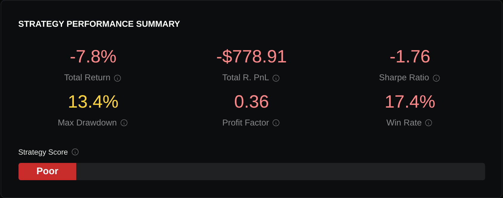
The worst neighbor trails the baseline by 1.0312 percentage points of return. This is a local comparison on one development window, not later validation, an untouched final test or proof of robustness. Commission charging and detailed signal/fill reconciliation remain unresolved; the screenshots and table report the product’s observed results under its configured settings.

Start with one existing strategy, write down a small neighborhood, and compare its completed runs under identical assumptions using the backtest setup guide. The next decision should follow the evidence you planned to collect.