Backtest one ETF trend filter across SPY, QQQ, and IWM

A moving-average filter asks a simple question: should this ETF be held, or should its account stay in cash? Testing the same rule across SPY, QQQ, and IWM helps you investigate whether the idea transfers across different equity exposures.

Keep the rule unchanged. Choosing a different winning average for every ETF answers a different question: how well can you fit three historical charts?

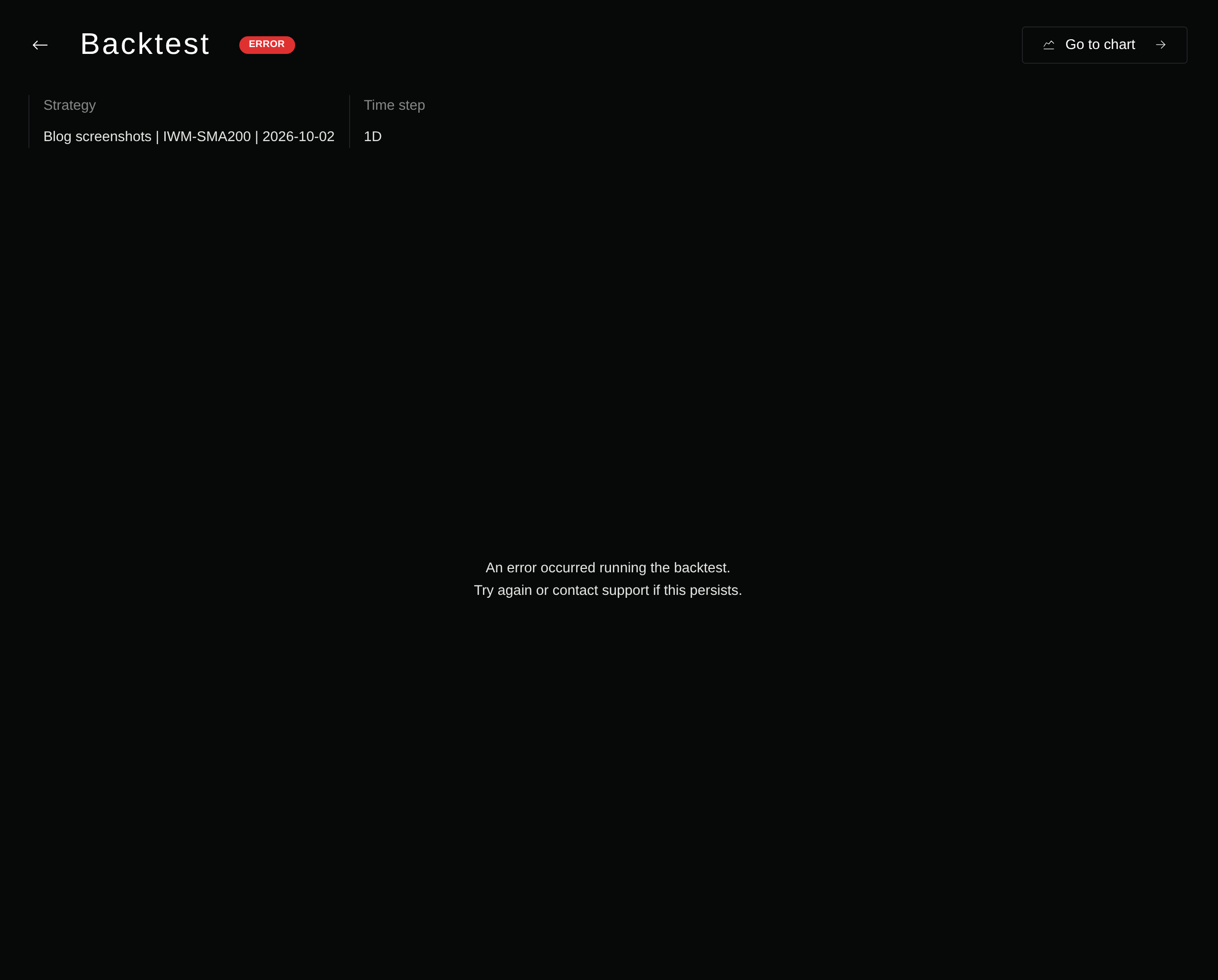
The specification below is a teaching experiment. The product captures use a separate shorter demonstration on January 2, 2024 through June 30, 2025: SPY and QQQ completed with the same 200-bar filter; IWM failed and returned no historical bars in the coverage check. These captures do not complete the two-window, three-fund research specification.

Start with three separate ETF accounts

The funds give the comparison different underlying exposures:

ETF	Exposure to compare
SPY	S&P 500 exposure, as described by State Street.
QQQ	Nasdaq-100 exposure: the largest non-financial companies listed on Nasdaq, as described by Invesco.
IWM	Russell 2000 exposure to U.S. small-cap stocks, as described by iShares.

Give each ETF its own hypothetical $10,000 account. Each account trades only its assigned ETF and holds its own cash. These are three independent experiments; their balances do not add up to a $10,000 portfolio.

A shared basket with one cash pool introduces capital competition. If several ETFs signal together, order priority and allocation rules can affect which positions open. Establish how the filter behaves independently before adding that portfolio question.

Define the filter as a position state

Use a 200-session simple moving average of closing prices. A simple moving average is the mean of its input prices; longer windows smooth more observations and respond more slowly. Fidelity identifies a 200-bar SMA as a common long-term trend measure. That convention does not establish an optimal period for these ETFs. Fidelity’s SMA guide.

For every completed daily bar:

• Calculate the SMA from the latest 200 trading-session closes, including that bar.
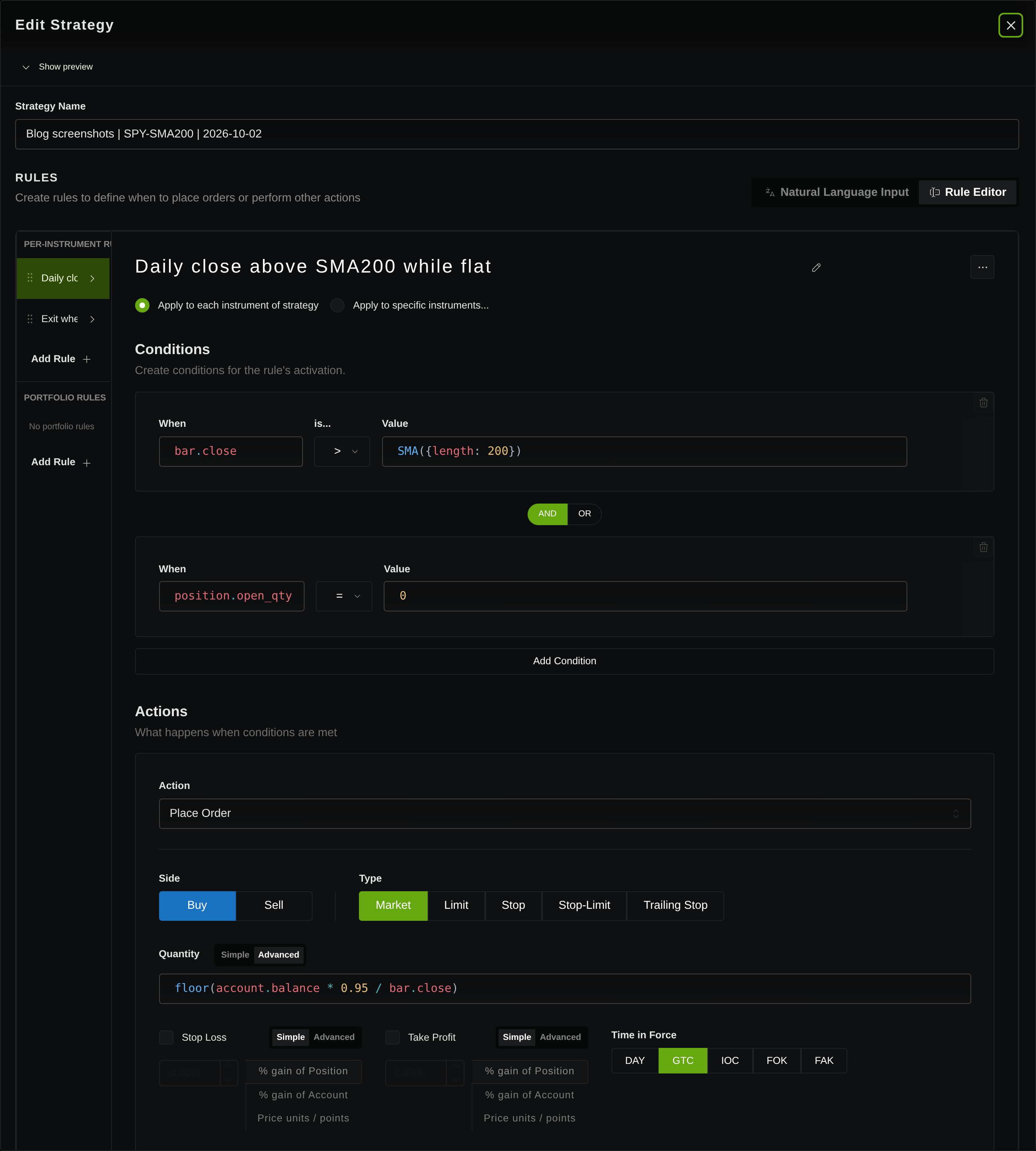
• If the close is strictly above the SMA and the account is flat, request a long entry.
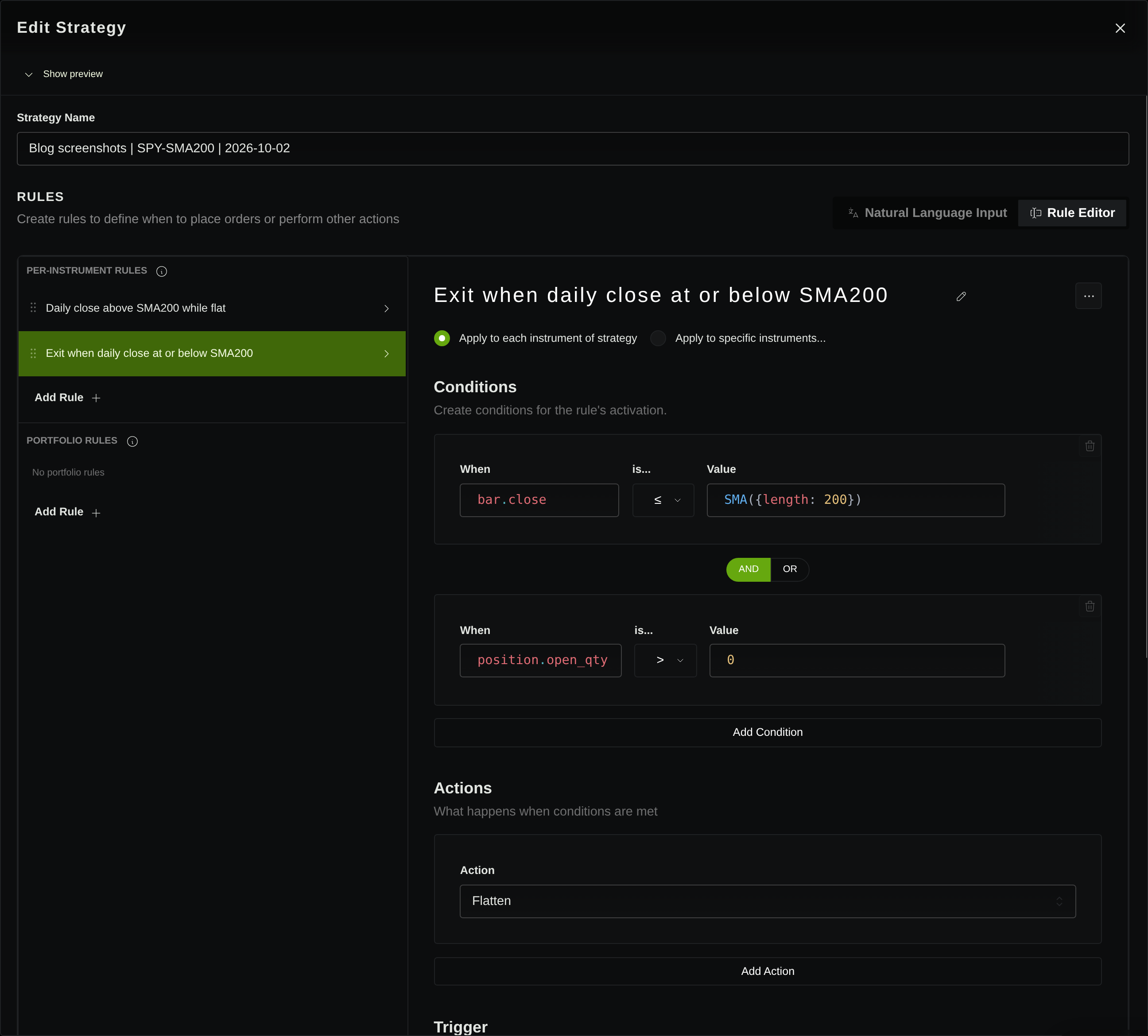
• If the close is at or below the SMA and the account holds shares, request a full exit.
• Otherwise, keep the existing state. Do not add another position while already long.

This is a price-above-average filter. It does not require a fresh crossing event. If the first eligible close is already above the SMA, the account can enter without waiting for a new upward cross.

Do not substitute 200 calendar days for 200 observations, or switch QQQ to an exponential average midway through the comparison. Keep the close series, window, equality rule, and position limit identical.

Require split-only adjusted closes for both the current close and the SMA inputs, on the same share scale at each evaluation. Leave dividends out of those price adjustments and account for eligible distributions separately as cash. Use unadjusted signal-day prices for quantity calculations and raw execution prices for fills; split events must update held share quantities consistently. Verify that the actual data and run implement this convention before interpreting the comparison.

Freeze the experiment settings

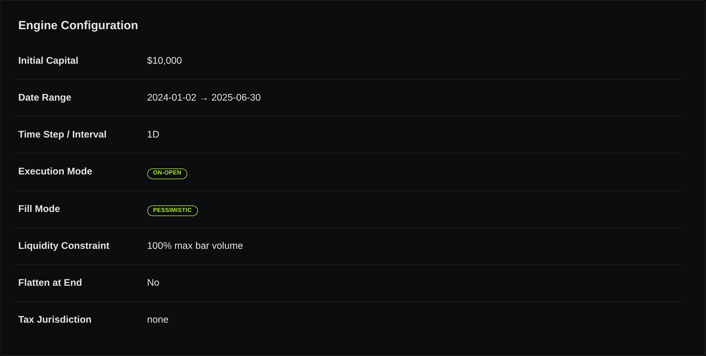
Write down a shared specification before running any ETF:

Setting	Teaching specification
Initial balance	$10,000 independently for each ETF and each baseline.
Review window	January 2, 2015 through December 31, 2019.
Later comparison window	January 2, 2020 through December 31, 2025; inspect only after freezing the first-window specification.
Bars and sessions	Daily regular-session bars, interpreted in America/New_York; honor holidays and early closes.
Warmup	At least 200 completed session closes available at the first evaluation; earlier observations generate no trades.
Signal price series	Split-only adjusted closes on one consistent share scale; no dividend adjustment.
Entry quantity	Whole shares: round down 95% of available cash divided by the signal day’s unadjusted close.
Intended execution	Evaluate the completed close; submit the fixed quantity for the next regular-session opening opportunity.
Trading costs	Hypothetical $1 per executed order plus 0.05% adverse slippage on each fill; these are experiment inputs, not quoted broker rates.
Exposure limits	One long position, no borrowing, no shorting, no stop-loss or profit target.
Cash	Zero interest; distributions remain cash until a subsequent permitted entry.
Window boundary	Mark open shares at the final regular-session unadjusted close; cancel pending orders, with no assumed liquidation fee.

The 5% reserve helps leave room for costs, but an overnight gap can still make the requested quantity unaffordable. Record rejections and partial fills. Do not silently add leverage, resize using a future price, or treat a requested order as a completed position.

Restart each window with the same initial balance and sufficient prior warmup. The later window is a check of the frozen rule, not a reason to choose a new average. Because both windows are historical, this procedure alone does not establish that your research was free of hindsight.

Prove the signal came before the fill

The intended sequence matters more than a setting called “open” or “close.” A daily close becomes known only after that session’s trading. A fill at that morning’s open cannot use that completed close.

Inspect the first entry and first exit against their underlying bars. Record the signal session, closing price, calculated SMA, order quantity, fill session, fill price, and charged costs. Confirm that the execution opportunity follows the completed signal bar and that the quantity used only information available when it was submitted.

If your run cannot establish that sequence, it has not tested the specification above. Preserve the observed behavior and correct the setup before comparing returns. A market-open fill is also a simulation assumption, not proof that a live order would receive the official opening price.

Give the baseline the same accounting

For each ETF, create an unfiltered holding baseline with the same $10,000 balance, start and end dates, price data, costs, and cash policy. Calculate its entry quantity at the first in-window completed close with sufficient warmup, then request its buy at the following regular-session open inside the window. That is also the earliest opening opportunity allowed for the filtered account. Hold the baseline’s shares through the window. It also leaves a reserve; do not compare it with a fully invested fund performance figure.

End both versions at the final regular-session close inside the window. Cancel pending orders, retain open shares, and value them at that session’s unadjusted close plus cash; charge no hypothetical liquidation fee. Skip final-session signals whose opening fill opportunity falls outside the window, and include only fills inside it. Label this result as account value with open positions. Closed-trade profit alone omits the risk and value of those shares.

Distributions need their own audit. State Street’s published SPY returns assume reinvestment of dividends and capital gains; iShares uses reinvestment in IWM’s hypothetical growth illustration. Those figures are not interchangeable with an account that keeps distributions in cash. SPY performance methodology, IWM performance methodology.

Verify split handling, the price adjustment convention, distribution entitlement, and cash-credit timing for the actual data and run. Do not combine dividend-adjusted returns with another credit of the same dividend. An engine’s ability to process an action does not prove every relevant ETF distribution reached this backtest. If distributions are missing, label the result as a price-only experiment and do not call it investor total return.

Compare exposure as well as return

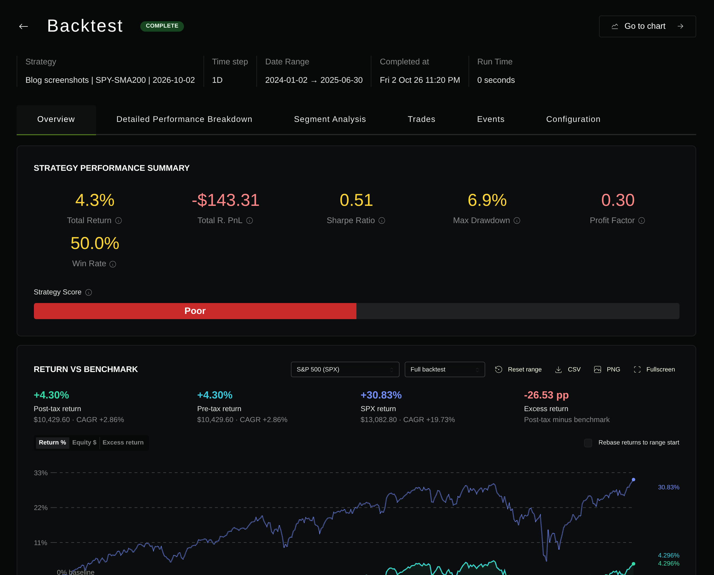
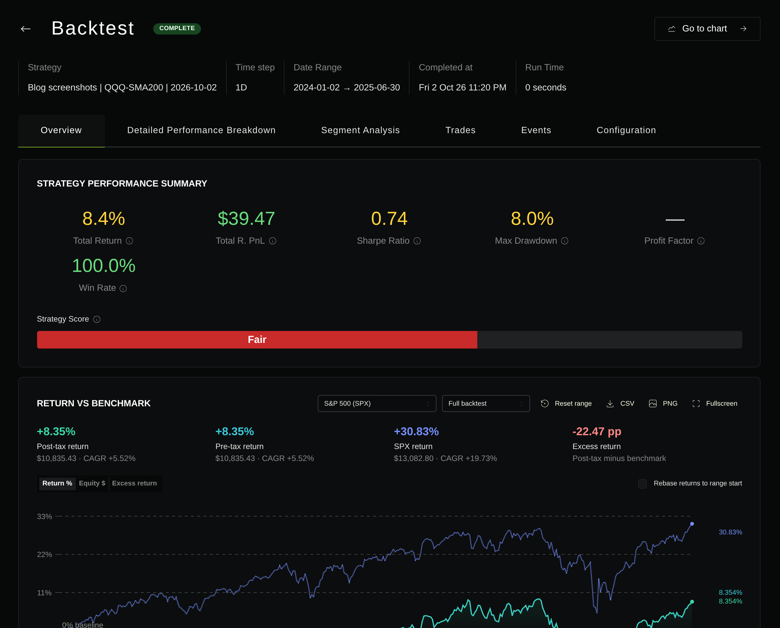
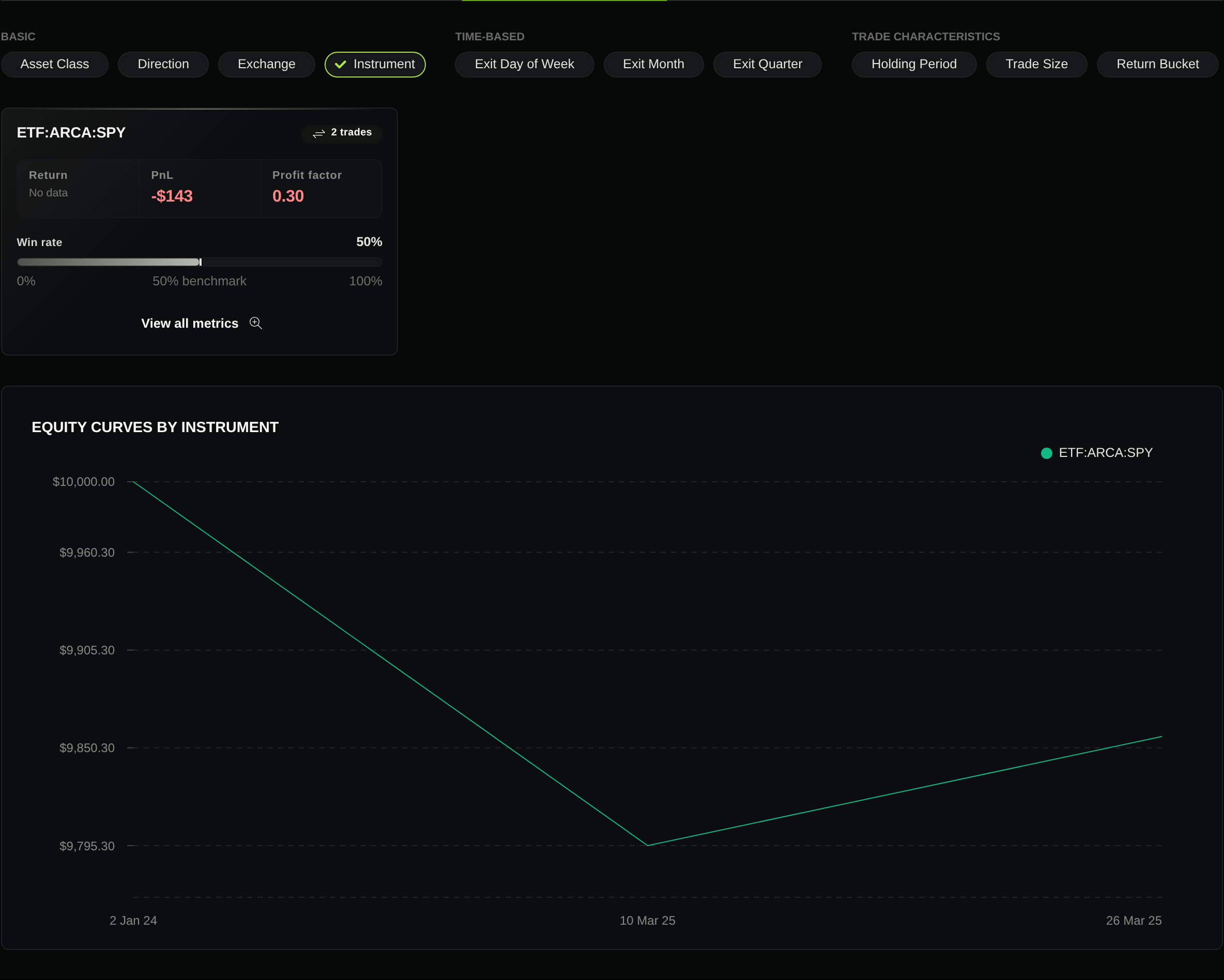
Make one record per ETF, showing filtered and baseline results side by side:

• Ending account value after costs: did the filter leave more or less money, including cash and open positions?
• Maximum drawdown and recovery time: how deep was the decline, and how long did the account take to regain its earlier high?
• Time invested: at how many eligible session closes did the account actually hold shares, divided by the number of eligible sessions?
• Average capital utilization: the average fraction of account value held in the ETF at those closes.
• Turnover and costs: how much buying and selling occurred, how many orders executed, and what did they cost?
• Distributions and cash: which credits occurred while eligible, and how much capital remained idle?

Time invested uses actual holdings, not the number of “above average” signals. Partial fills and pending exits can separate those counts. Capital utilization adds another distinction: a partly invested account can hold shares every session without deploying its full balance.

Inspect a whipsaw: an exit followed soon by re-entry that incurs costs without avoiding much downside. Inspect a prolonged cash interval too, including rallies missed before the next permitted entry. These observations explain a curve more clearly than declaring whichever ETF finished highest the winner.

Keep the conclusion narrow

Ask whether one unchanged filter produced a useful trade-off between drawdown, idle capital, turnover, and ending value across all three ETFs and both windows. Keep unfavorable outcomes in the comparison. SPY, QQQ, and IWM still represent related equity exposures; agreement among three funds is not broad proof of diversification or future performance.

AQR’s long-history trend-following research studies a broader strategy across several markets, including long and short exposures. It provides context for investigating trends, not validation of this long-or-cash ETF rule. AQR’s original research.

Use the Stratifyre backtesting guide to prepare one fixed rule for the three ETF tests, then inspect the first entry and exit before interpreting performance.