Walk-forward backtesting example: one rule, three folds
Choose strategy settings on earlier data, test them on the next window, and combine the results without double-counting dates or confusing capital with position carry.
A walk-forward backtesting example starts with a simple restriction: choose the settings using earlier prices, freeze them, then test on the next window. Repeat the same procedure as time advances. The question is whether your selection process survives later data, rather than which settings make the whole historical chart look best.
The daily-equity strategy specification, timeline, and arithmetic below are teaching examples, not executed backtest results. A separate completed Bitcoin demonstration at the end shows the actual product workflow with shorter windows and different rules.
Freeze one rule and three candidates
Use a crossover of simple moving averages (SMAs) of completed daily closing prices as the teaching rule. Keep the slow SMA at 120 bars; test fast SMAs of 20, 40, and 60 bars. Enter long when the fast SMA crosses from at or below the slow SMA to above it. Exit when it crosses from at or above to below. Allow one position and no shorts.
Write the rest of the experiment before seeing any results:
- Market and data: one chosen equity ETF, one unchanged historical dataset, regular-session daily OHLC bars, and the instrument’s exchange calendar. Record the exact instrument ID, data source, timezone, and split/dividend treatment before running; use a consistent adjustment convention across indicators and fills.
- Timing: evaluate after the daily close; ordinary orders fill at the next regular-session open inside the same window. A close signal cannot use that day’s earlier opening price.
- Sizing: start with $10,000 cash, allocate at most 90% of available cash to an entry, round down to whole shares, and leave room for costs. No leverage or pyramiding.
- Costs: assume 5 basis points of commission and 5 basis points of adverse slippage on each fill. These are teaching assumptions, not a broker quote. Use the same assumptions for every candidate and fold.
- Window boundaries: start every child run flat, carry no pending orders into the next child run, and close remaining exposure at the last available in-window close with costs. Label this forced close separately from a normal exit.
Choose one training score in advance: for this example, maximize net return after the stated costs, with ties resolved in the order 20, 40, then 60. This is a deliberately simple selection rule; it can favor riskier candidates. Inspect drawdown and trade count alongside it, but do not switch objectives after inspecting test results.
Draw the train, select, test timeline
Each fold contains a training window, a selection step, and a later test window. Training is in-sample (IS); testing is out-of-sample (OOS) relative to that fold’s selection.
Chronological order matters: scikit-learn’s TimeSeriesSplit documentation explains why ordinary cross-validation can train on future observations and evaluate on the past. Its default expanding training sets illustrate anchored testing; a fixed-length rolling window is a separate geometry choice.
Use 24 months of training, six months of testing, and a six-month step:
| Fold | Training [start, end) |
Test [start, end) |
|---|---|---|
| 1 | 2021-01-01 → 2023-01-01 | 2023-01-01 → 2023-07-01 |
| 2 | 2021-07-01 → 2023-07-01 | 2023-07-01 → 2024-01-01 |
| 3 | 2022-01-01 → 2024-01-01 | 2024-01-01 → 2024-07-01 |
[start, end) includes the start and excludes the end. January 1, 2023 belongs to fold 1’s test, not its training. Calendar boundaries apply even when a boundary date is a holiday; trade only on available sessions inside the window. The combined test coverage is January 2023 through June 2024. The initial training period contributes no OOS returns.
In rolling testing, both training boundaries move forward. In anchored testing, the training start stays at January 2021, while the training end advances. Here, anchored training would grow from 24 to 30 to 36 months. Choose the geometry before running; trying both and retaining the prettier test curve adds another research trial.
Fold 1’s test dates can later enter fold 2’s training: those observations would be historical by then. That is consistent with a prespecified retraining schedule. It does mean the folds share information and should not be treated as independent experiments.
Select inside training; initialize without looking ahead
For each fold, run all three candidates on its training window with identical assumptions. Save the candidate scores and select the highest training score. Run only that selected configuration on the following test window. Retain every fold’s output, including losing or inactive folds.
Warmup is different from training. Moving averages need prior completed bars to initialize; a crossover also needs a previous comparison. For this teaching rule, require at least 121 completed daily bars of prior history before the first evaluated close. Check that the loader actually supplies them. If history is missing, record the delayed evaluation start and reduced test coverage rather than pretending the indicator was ready.
Earlier training bars may initialize a test-window indicator because they were already known. They must not generate test-window trades or returns before the test starts. Never initialize with a future bar, use a full-window statistic that includes later prices, or select parameters using the upcoming test score.
Position state needs its own decision. This recipe resets exposure between child runs and charges forced exits. That changes turnover and may cut a trend short. Passing the previous fold’s ending cash into a new run does not also carry its shares, entry price, or pending orders. A continuous-position experiment requires different boundary rules and should not be compared as though it were identical.
Combine only the test windows
Keep the three OOS windows in time order, exclude all training curves, and check that no date is counted twice or silently omitted. Then identify the capital convention.
Fixed capital: every test starts with $10,000. Combine its dollar gain or loss with the preceding folds’ gains or losses. This describes repeated tests with equal starting capital.
Rolling capital: the next test starts with the previous test’s ending equity. The cash basis changes, and position sizing must use that changing basis.
Consider hypothetical net OOS returns of +5%, −4%, and +3%, invented only to demonstrate the arithmetic:
| Convention | Calculation | Teaching endpoint |
|---|---|---|
| Fixed | $10,000 + $500 − $400 + $300 | $10,400; +4.00% |
| Rolling | $10,000 × 1.05 × 0.96 × 1.03 | $10,382.40; +3.824% |
The arithmetic differs even with the same percentage inputs. Real runs can differ further because share rounding, costs, and constraints interact with capital. Averaging the three percentages does not produce the compounded total return.
Endpoints cannot show the path’s worst drawdown. Rebuild drawdown from the combined dated equity series under the chosen capital convention; an average of fold drawdowns is a different quantity.
Read stability before redesigning
For each fold, record the selected fast-average length, training score, OOS net return, drawdown, trade count, exposure, and forced exits. Include periods with no trades. Compare candidates’ training scores: a tiny advantage supported by a few trades gives little reason to believe one setting is clearly better.
Then inspect whether test behavior depends on one strong period, whether losses cluster, and whether the chosen parameter jumps between extremes. Stable parameters are useful context, but do not establish an edge. Prespecify a separate higher-cost scenario if you want to examine execution sensitivity; report it alongside the baseline rather than selecting the better outcome.
Repeatedly changing the rule after seeing these test windows makes them part of your research history. Bailey and colleagues’ The Probability of Backtest Overfitting explains why investment holdouts and multiple strategy trials can still produce misleading selection. Walk-forward testing does not erase all those trials or calculate that paper’s probability of overfitting.
Keep a trial log, preserve unsuccessful designs, and reserve later untouched data for evaluating a revised process. A useful result can be a reason to stop: sparse trades, unstable choices, missing warmup coverage, or losses after costs all answer the original question.
Actual product example: three monthly Bitcoin folds
We also executed a smaller demonstration in a dedicated demo account: Binance BTC/USDT hourly bars, January through April 2025, three rolling folds with one month of training followed by one month of testing. This is a different experiment from the daily-equity recipe above. It buys 0.05 BTC when the entry EMA crosses above EMA(50) while flat; the exit remains EMA(20) crossing below EMA(50). Only the entry EMA length varies across 18, 20, and 22 bars. Each child run starts with $10,000, uses on-open execution, pessimistic fills, final flattening, 0.10% configured crypto commission and 0.05% slippage. Configured commission is not proof that every fill was charged correctly.
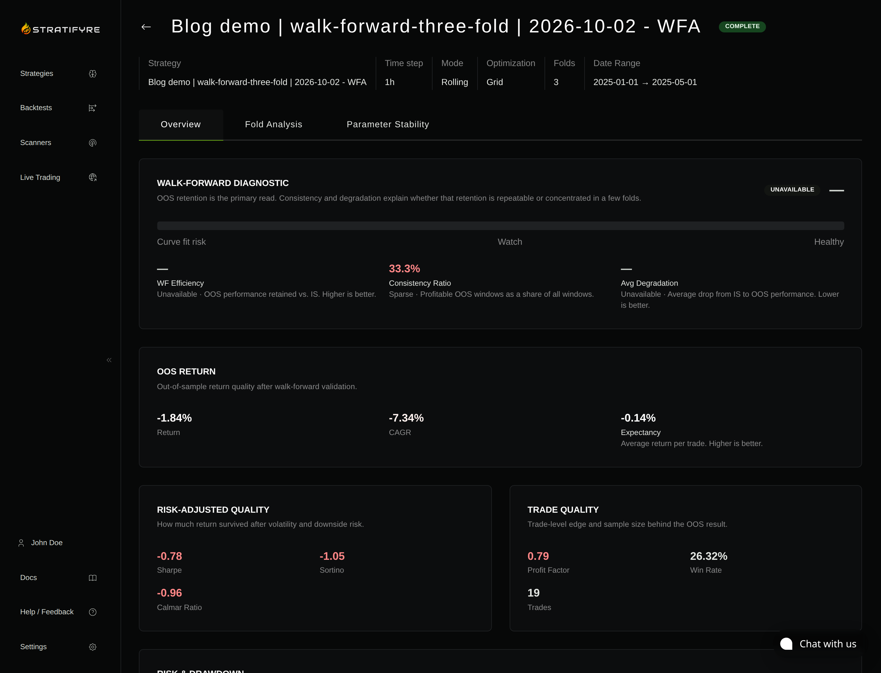
Training selection maximized return and retained every candidate. The selected lengths moved from 18 to 20 to 22; all three selected training returns were negative.
| Fold | Training [start, end) |
Test [start, end) |
Entry EMA selected | Training return | Test return | Test trades |
|---|---|---|---|---|---|---|
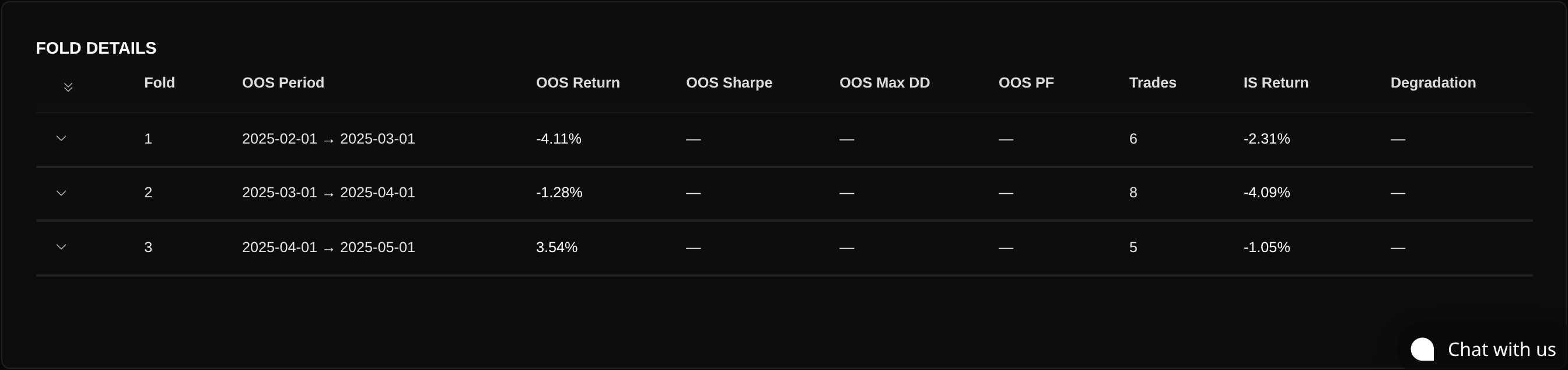
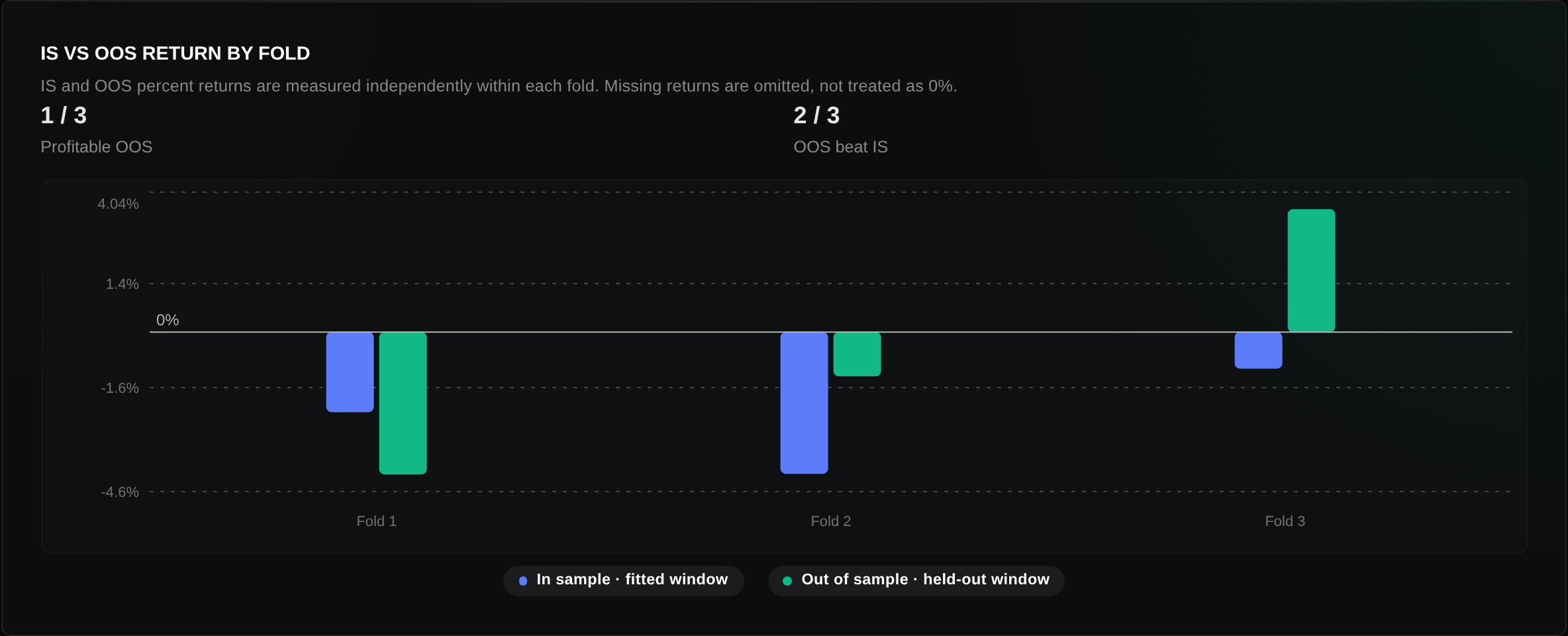
| 1 | 2025-01-01 → 2025-02-01 | 2025-02-01 → 2025-03-01 | 18 | −2.3106% | −4.1061% | 6 |
| 2 | 2025-02-01 → 2025-03-01 | 2025-03-01 → 2025-04-01 | 20 | −4.0867% | −1.2758% | 8 |
| 3 | 2025-03-01 → 2025-04-01 | 2025-04-01 → 2025-05-01 | 22 | −1.0532% | +3.5423% | 5 |
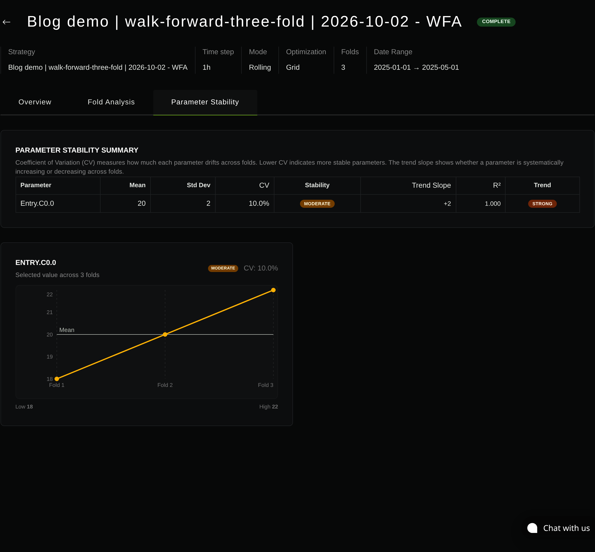
Entry.C0.0, the entry EMA length. The exit EMA and position quantity remained unchanged.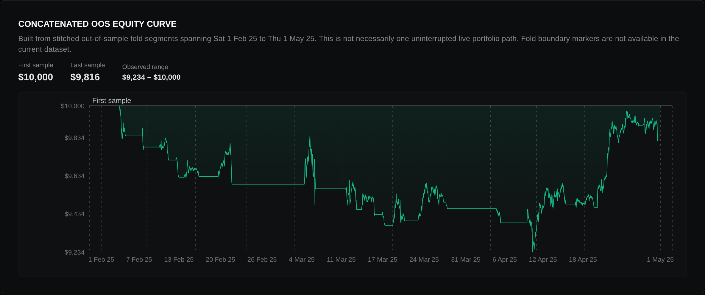
The screenshots establish this completed demonstration, not the longer ETF experiment or a fully reconciled execution model. The product reports missing fold-level Sharpe, drawdown and profit-factor values, while aggregate values are available. Opening an OOS child ID through the ordinary backtest route returned “Backtest not found”; the retained WFA report and variant records supply the actual evidence. Warmup coverage, individual fill costs and exact boundary-fill reconciliation still require separate checks.
For a first experiment, use Stratifyre’s walk-forward testing overview to plan one small candidate set with prespecified folds. Verify the actual rules, warmup coverage, fills, boundary exits, capital mode, and child-run outputs before interpreting an OOS curve.
Put your strategy rules to the test
Build your strategy, inspect historical trades, and review the assumptions behind your results.
Build and test your strategy