Does your strategy behave differently in high volatility?
Compare one unchanged strategy across conditions known at entry, using explicit volatility labels, real trade counts, and careful timing.
An overall backtest hides the conditions surrounding its trades. A strategy might collect most of its gains during large price swings, while smaller moves produce repeated reversals. Market regime analysis asks whether those outcomes differ under a definition you can apply consistently.
The timing matters as much as the definition. A condition measured after a trade closes cannot explain what was knowable when you entered. Start with one unchanged strategy, label each entry using earlier completed prices, and keep every trade in the comparison.
In the selected Bitcoin example below, higher entry volatility accompanies a larger average recorded profit. Both groups finish positive, and the sample contains only 19 trades. That is a historical observation to investigate, not evidence that a high-volatility filter would improve future trading.
Keep the strategy fixed
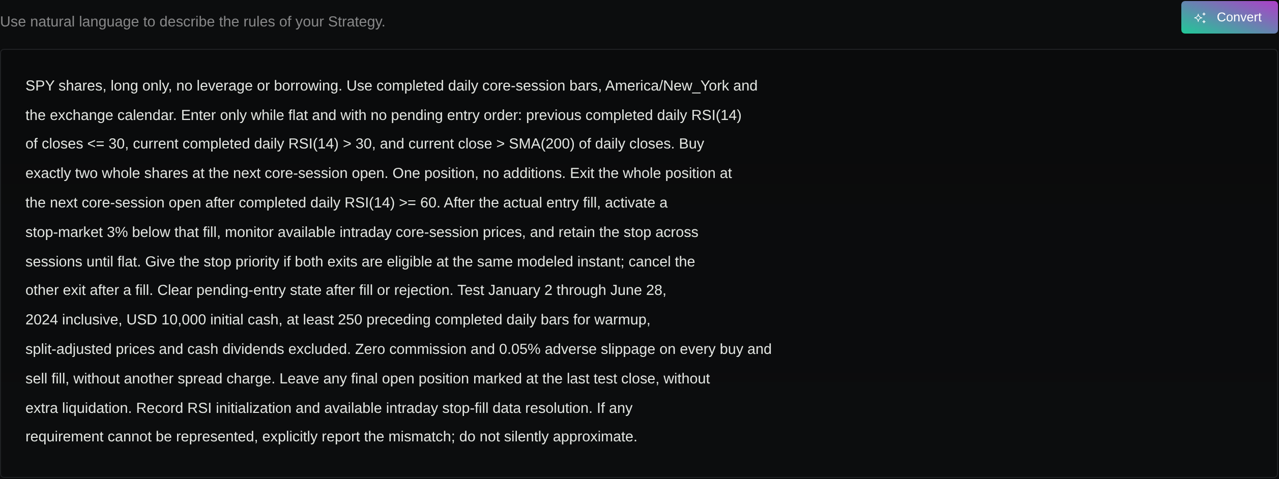
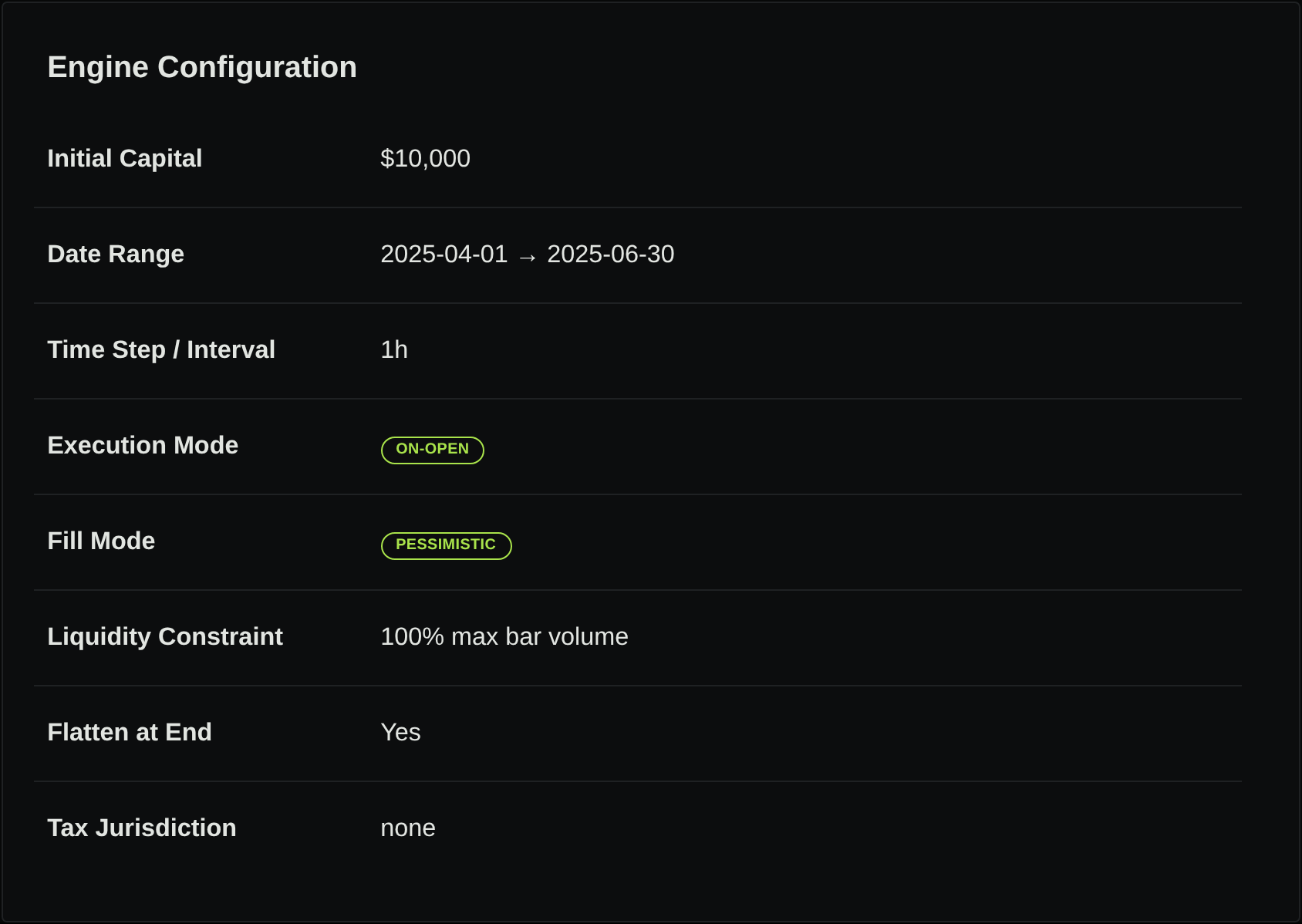
We reused a completed Binance BTC/USDT hourly backtest covering April 1–June 30, 2025. Its rules bought 0.05 BTC when EMA(20) crossed above EMA(50) while flat, then flattened the position on a downward crossover while holding BTC. Capital started at $10,000; execution was configured as on-open, with pessimistic fills, 0.05% crypto slippage, and flattening at the end.
The report contains seven winners and twelve losses, totaling +$958.09 recorded trade P&L. The configured 0.10% crypto commission returned zero fees in every retained trade. These figures therefore do not establish performance after that commission, even though the report is complete.
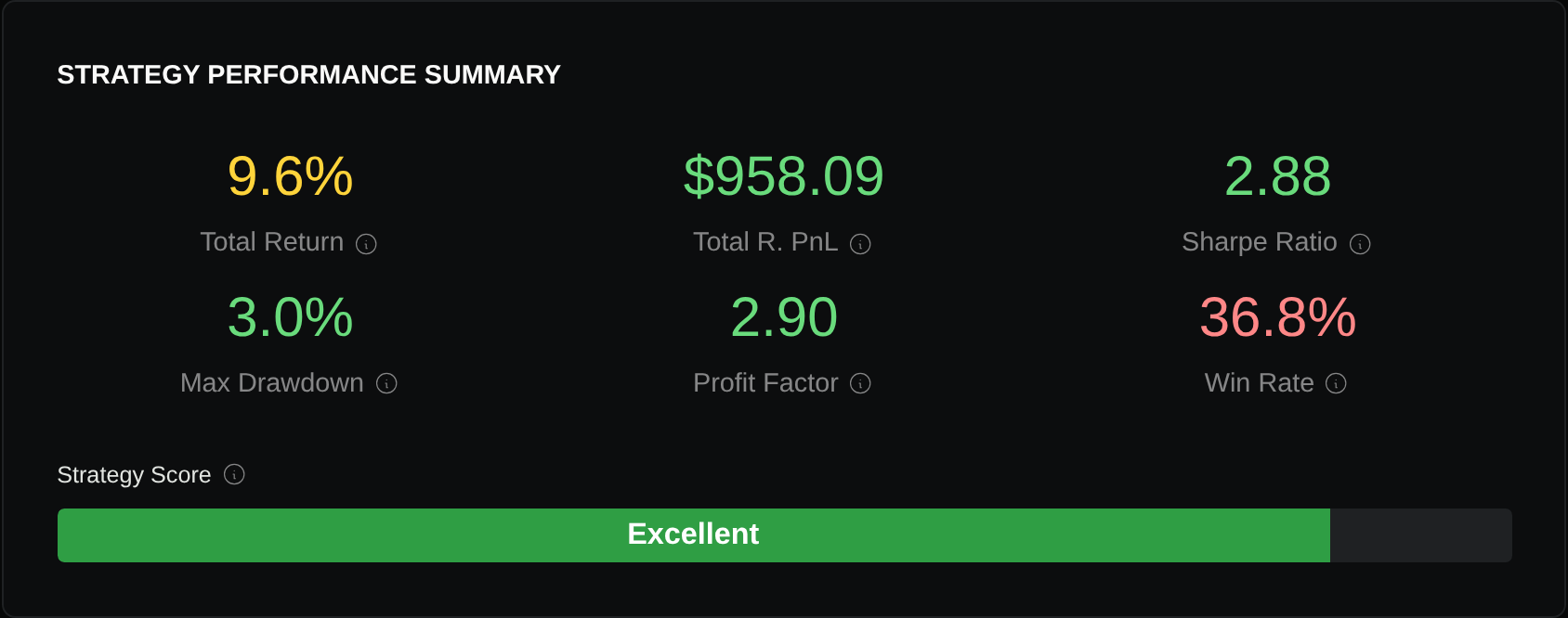
This quarter was already selected as a profitable example for our profit-concentration article. We knew its trade outcomes before defining the volatility labels. We fixed the formula and threshold before calculating those labels, but this remains retrospective analysis of a selected historical result.
Define volatility using prices available at entry
For each recorded entry, we took 25 consecutive completed hourly closes, producing 24 hourly log returns. We calculated their sample standard deviation, multiplied it by √24, and expressed the result as a percentage. This is our trailing 24-hour volatility proxy; it describes recent movement without forecasting the next day or its direction.
Hourly return: r = log(current close / previous close)
Volatility proxy: 100 × sample standard deviation of 24 returns × √24
Lower: below 2%. Higher: 2% or above.
The 2% boundary is an author-chosen convention for this example. It is neither a native Stratifyre classification nor an optimized threshold. We did not move it after seeing which group earned more.
An hourly candle stamped 19:00 UTC spans the following hour. For a 20:00 entry, that candle’s close is eligible; the 20:00 candle’s eventual close is excluded. The earliest close supplies the starting price for the first return, which is why 24 returns require 25 closes. If a required close is missing, record the trade as unclassified instead of filling the gap silently.
Our product-data request returned 2,016 consecutive hourly bars from April 2 through June 24, 2025, sufficient for every recorded entry from April 4 through June 23. All 19 trades had complete inputs; none were excluded. The analysis retains 463 distinct closes across their overlapping windows. These are bars fetched after the original execution, so historical data revisions remain a possible difference from the original run.
Compare counts before comparing totals
The unchanged strategy produced the following groups. Dollar figures use the recorded trade P&L, with the commission limitation above; winning and losing counts depend on that same P&L sign. The labels describe conditions at entry, while each profit or loss spans the entire holding period.
| Entry volatility | Trades | Winners / losses | Recorded P&L | Mean per trade | Profit factor |
|---|---|---|---|---|---|
| Lower: below 2% | 10 | 2 / 8 | +$199.15 | +$19.91 | 1.50 |
| Higher: at least 2% | 9 | 5 / 4 | +$758.94 | +$84.33 | 8.05 |
| All trades | 19 | 7 / 12 | +$958.09 | +$50.43 | 2.90 |
Profit factor here divides positive recorded P&L by the absolute value of negative recorded P&L. There were no zero-P&L trades. The group totals reconcile to the full trade list without changing the strategy or removing losses.
Different historical averages, very small samples
View example data
| Entry group | Mean recorded P&L ($) |
|---|---|
| Lower | 19.91476985 |
| Higher | 84.32658581 |
The higher group still includes four losses. For example, the April 4 entry had a trailing proxy of 3.55% and recorded a $66.90 loss. Conversely, the April 21 entry had a 1.18% proxy and became the run’s largest winner, earning $431.62. A group average does not make every entry in that group attractive.
Native exit segments answer a different question
Stratifyre’s native time segments include Exit Day of Week, Exit Month, and Exit Quarter. They group completed trades by their UTC exit timestamp. In this run, the Exit Month totals were April +$353.61 across six trades, May +$487.08 across seven, and June +$117.39 across six.
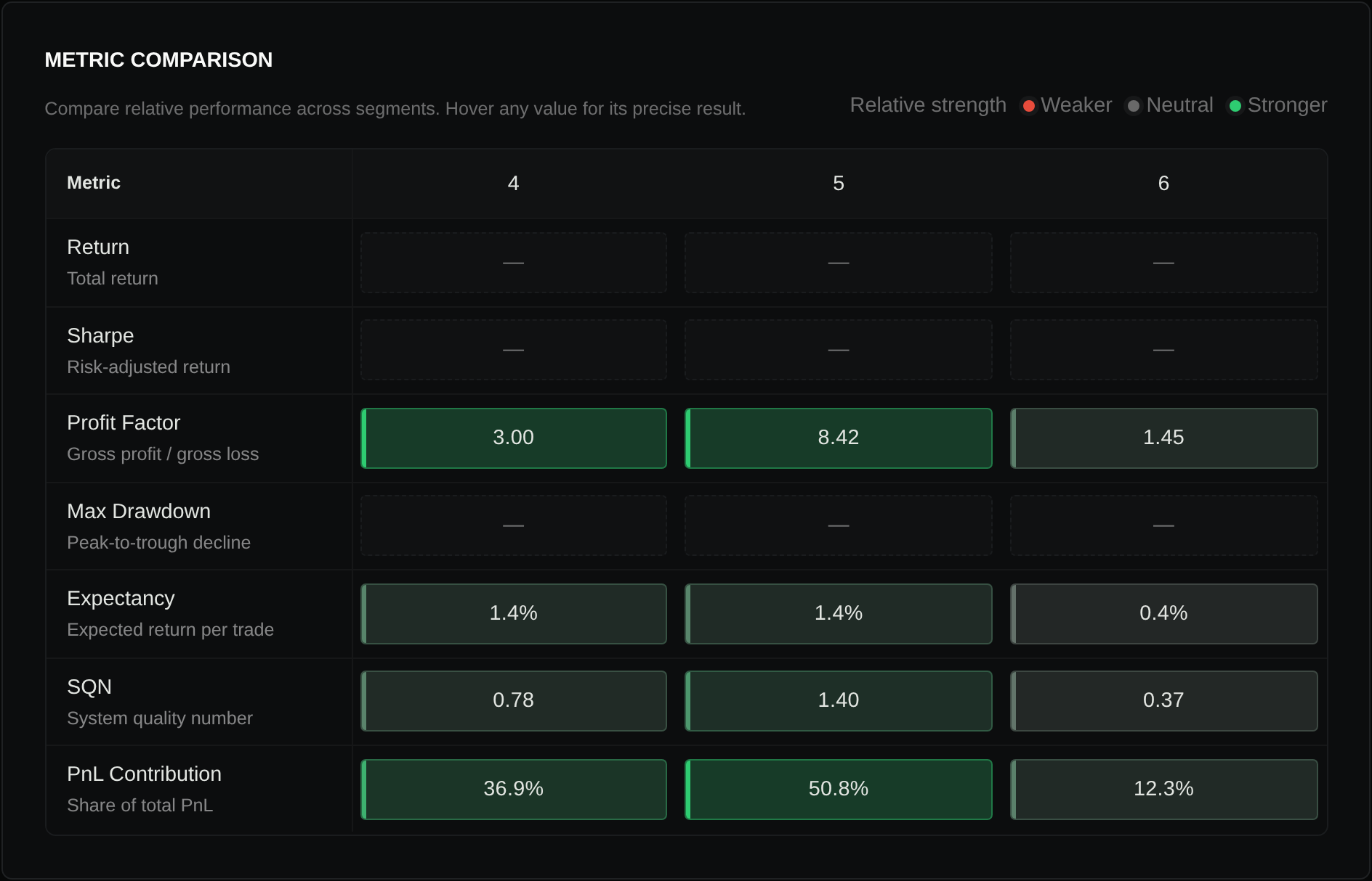
An exit-month result tells you when completed trade P&L was attributed. It does not establish which conditions were present at entry. Similarly, grouping trades by their eventual return identifies outcome sizes; it cannot provide a condition known before taking the trade.
Turn the observation into a new test
Nine and ten trades are too few to establish a dependable regime effect. Trades share one instrument and one quarter; overlapping volatility windows are not independent experiments. Fixed 0.05 BTC quantity also gives different dollar exposure as price changes, so these averages are not an equal-risk comparison.
Volatility can change after entry. We held each entry label fixed, rather than relabeling a trade as market conditions evolved. This analysis neither measures time spent in each regime nor estimates marked-to-market drawdown for separate regime portfolios. It also does not revalidate the original indicator warmup or chart-to-fill replay timing.
A useful next experiment would freeze the same labels and unchanged rules for an untouched window, keep all outcomes, and reconcile actual charged costs. If you then propose a volatility entry filter, test it as a new strategy with its own cash, skipped signals, and trade sequence. Subtracting one group’s trades from this report cannot reproduce that execution.
Avoid repeatedly trying boundaries until a historical split looks convincing: searching many variants on the same data can produce false discoveries, as discussed in Bailey and colleagues’ original backtest-overfitting research. We have not calculated an overfitting probability or statistical significance for this example.
Start by inspecting the available performance segments and writing down exactly which timestamp each uses. Preserve that distinction when adding your own entry-time labels, then use a separate evaluation window to test the resulting hypothesis.
Put your strategy rules to the test
Build your strategy, inspect historical trades, and review the assumptions behind your results.
Build and test your strategy